Goalie Performance: Empirical Bayes Adjusted Save Percentage

[Post 2] Goalie Performance: Empirical Bayes Adjusted Save Percentage

In the first post, I outlined a framework for measuring goalie talent using their career Fenwick 5v5 save percentage. It concluded with the assumptions of the initial strategy, which I'll include again below.

Assumptions: - All shots are assumed to be equal. - Age is assumed to be irrelevant. - The prior distribution is assumed to be beta with hyperparameters 852 and 55.6. - Goalies facing less than 200 shots are ignored. - Goalie careers are equal. - Scoring rates are assumed to be constant. - Team systems are assumed to be identical.

In this post, I'm going to address the first assumption and propose an adjustment.

Adjusted Save Percentage

All shots are not equal, in that they do not have the same probability of becoming a goal. This is established. Many Expected Goals (xG) models have been developed to account for this. Fortunately, Peter Tanner's website MoneyPuck provides detailed data on each unblocked shot in the NHL, including the probability of the shot being a goal according to his logistic regression model.

To adjust a goalie's save percentage for shot quality, we can incorporate these expected goal probabilities from MoneyPuck. Usually, after accounting for shot quality, goalie performance is measured by the number of goals saved above expected (GSAx). This changes the metric from a rate (percentage of shots saved) which is bounded by 0 and 1 to one that can include any real number. Unfortunately, the beta distribution only works with rates. One approach to retain the metric as a rate, and thus the beta distribution as a prior, is as follows:

- Fenwick Save Percentage (FSV%) = 1 - (Goals Against / Fenwick Shots Against) - Expected Fenwick Save Percentage (xFSV%) = 1 - (Expected Goals Against / Fenwick Shots Against) - Median Save Percentage (MSV%) = Median of Goalie (20+ xG faced) Career Save Percentage - Adjusted Save Percentage (AdjSV%) = MSV% + (FSV% - xFSV%)

Let's plot the distribution of career AdjSV% for goalies who have faced 200+ shots. We will also include a fitted beta distribution in white, and a weibull in red.

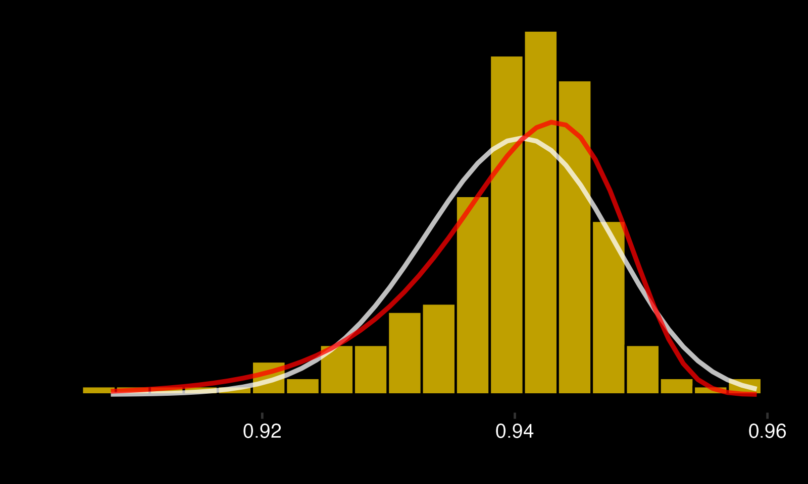
At first glance, goalies' career AdjSV% seems to follow a weibull distribution! Cool, but we're going to sidestep this finding for the remainder of the post, because (hint, hint) there maybe be more than one distribution here. So we're fitting another beta, which means the remaining steps remain the same as the previous post. The prior is similar, except this time we add 933 saves and 60 goals (up from 852 and 55.6).

Let's revisit the Jake Oettinger and Jeremy Swayman comparison.

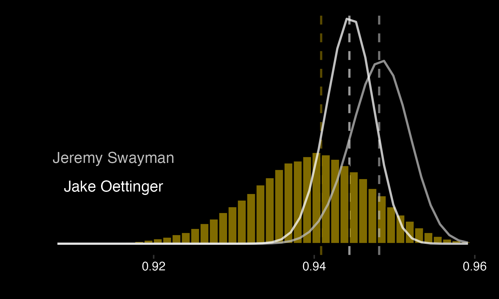
The posteriors change as follows: - There's a 78.77% (previously 60.28%) chance that Swayman's AdjSV% is better than Oettinger's. - There's a 88.28% (previously 94.12%) chance that Oettinger's AdjSV% is better than the MSV%. - There's a 97.30% (previously 93.81%) chance that Swayman's AdjSV% is better than the MSV%.

These changes occur because Swayman faces more difficult shots on average, with an xFSV% of 94.07 compared to Oettinger's 94.39.

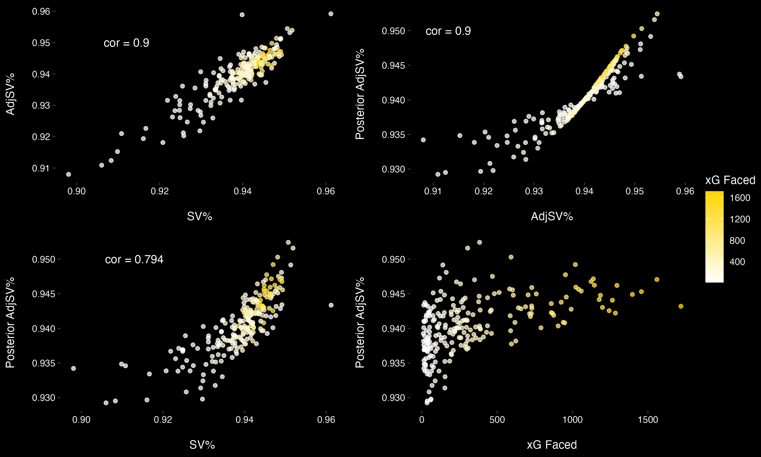
Appendix

Below is a collection of plots which compare various save percentage metrics discussed in this and the previous post.

A couple of key points: - Goalies who have a poor start to their career tend to play fewer games (surprise, surprise). - The relationship between a goalie's SV% and their AdjSV% seems to strengthen as they face more shots. - A goalie's AdjSV% converges with their posterior AdjSV% as they face more shots (indicated by the yellow diagonal line). - Due to the previous points, there is heteroskedasticity in the relationship between a goalie's SV% and their posterior AdjSV%. - There is likely survivorship bias present.

In the next posts, I'll adress the outstanding assumptions listed at the start.

Code available here: https://github.com/spazznolo/goalie-performance/blob/main/posts/post-2.R