[Post 1] Goalie Performance: Empirical Bayes Save Percentage

Recall from the introductory paragraph of the series on goalie consistency: "Goaltenders make up the least predictable position in hockey. Their behavior confounds analysts and casual fans alike. It isn’t uncommon for a good goalie to have a below replacement level year, or for an unknown goalie to come in and dominate the league for a stretch of time. This may partly explain the relative dearth of analysis on goalies - they're voodoo, it's often said."

This new series focuses on goalie performance. It aims to enhance the estimation of goalie performance using an empirical Bayes framework. Similar applications were outlined in previous papers. The strategy has several advantages over frequentist methods, chiefly the ability to measure uncertainty, which is crucial in describing goalie performance. In this post, the idea is sketched using raw save percentage as the performance metric, with further refinement of the methodology in subsequent posts.

The empirical Bayes approach involves two steps. The first step is to use observed data to fit a prior distribution, and the second step is to update this prior using observed data.

Step One

*Fenwick save percentage refers to the total percentage of unblocked shots saved, including shots that miss the net. It has been established that goalie skill correlates with the ability to make players miss the net.

To represent the possible career Fenwick save percentage for a new goalie, we can utilize the provided histogram of career 5v5 Fenwick save percentages for goalies who have faced 200+ shots (including those facing less adds noise - don't worry, it'll be addressed in a future post).

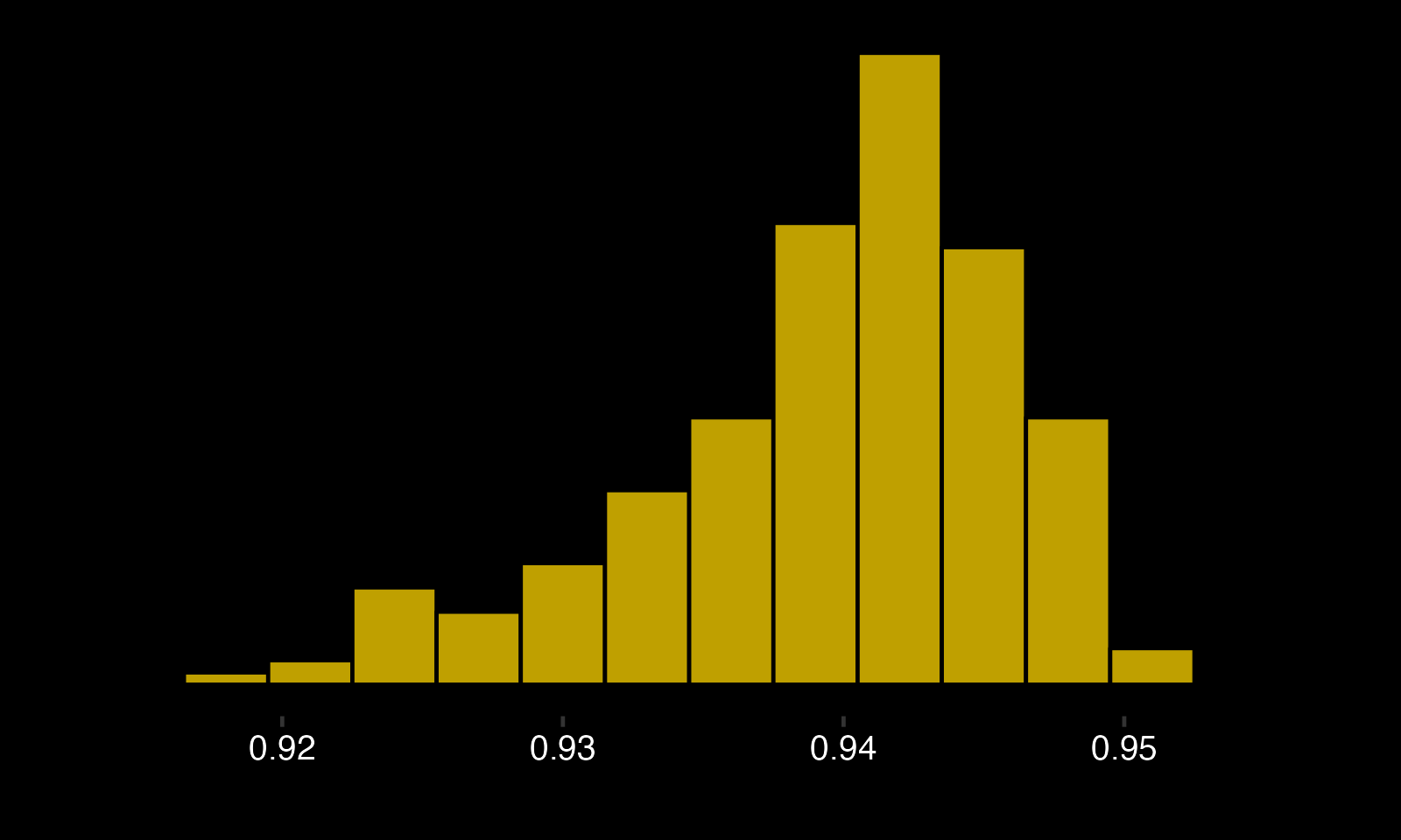
While the histogram provides a rough distribution, it contains random bumps throughout. To obtain a more structured representation, we fit a distribution to it.

The beta distribution is a commonly used prior when the variable of interest is a percentage, as in the case of the raw save percentage. Fitting a beta distribution to the career Fenwick save percentage distribution yields the following result.

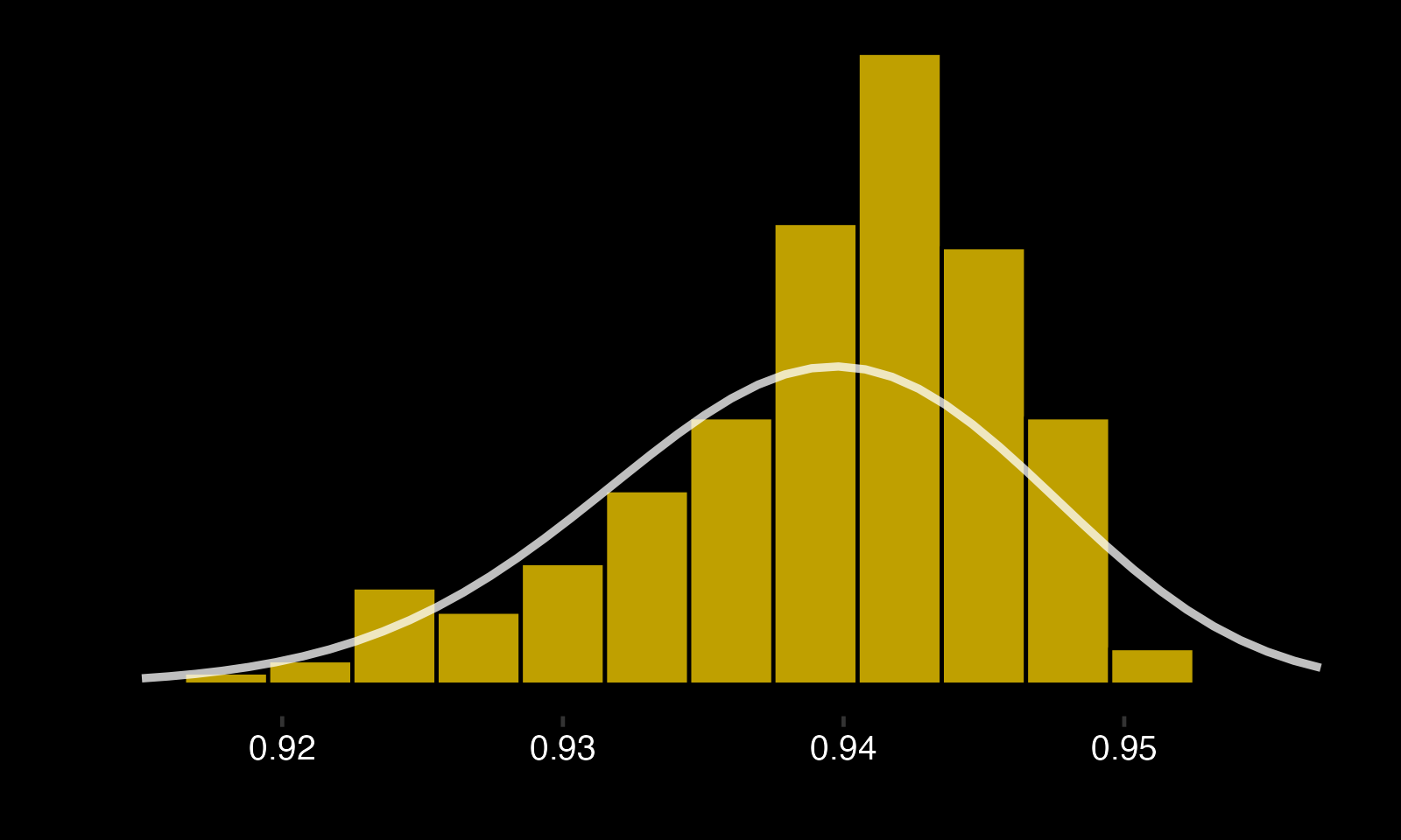
The fit is... not really good, and alternative distributions such as gamma or Weibull will be explored in future posts to find the best fit, but it serves its purpose as an introduction to the framework. The beta distribution has two hyperparameters, alpha and beta, which can be interpreted as successes (saves) and failures (goals). The fitted beta distribution in this case has hyperparameters 852 and 55.6, indicating that we attribute 852 saves and 55.6 goals to a goalie before knowing anything about them. This corresponds to a .9388 Fenwick save percentage, or, a little below the median save percentage for goalies facing 200+ shots (.9406).

Step Two

Updating the prior with observed goalie results is relatively straightforward. It requires adding the observed successes and failures (saves and shots) to the hyperparameters of the beta distribution.

As an example, let's plot the posterior distributions for two 24-year-old goalies: Jake Oettinger and Jeremy Swayman.

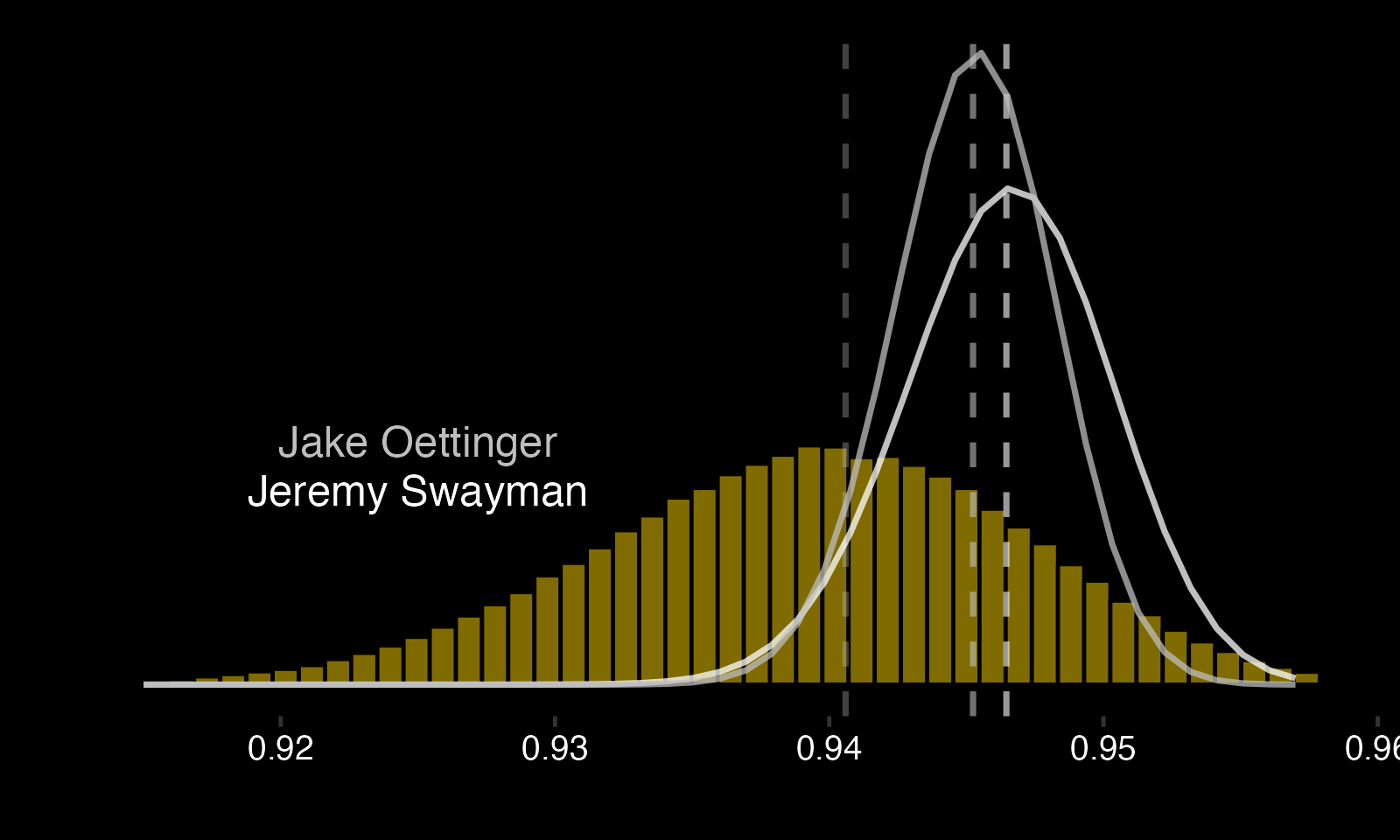
These posterior distributions offer interesting insights, like: - There's a 60.28% chance that Swayman's save percentage is higher than Oettinger's. - There's a 94.12% chance that Oettinger's save percentage is higher than average. - There's a 93.81% chance that Swayman's save percentage is higher than average. - Oettinger's distribution is tighter than Swayman's because he's faced more shots.

It's important to list all the assumptions with this method: - All shots are assumed to be equal. - Age is assumed to be irrelevant. - The prior distribution is assumed to be beta with hyperparameters 852 and 55.6. - Goalies facing less than 200 shots are ignored. - Goalie careers are equal. - Scoring rates are assumed to be constant. - Team systems are assumed to be identical.

These will be challenged and addressed in the following posts.

Code available here: https://github.com/spazznolo/goalie-performance/blob/main/posts/post-1.R