[Post 4] Goalie Performance: Exploring the Distribution

In the first post, I outlined a framework for measuring goalie performance using their career Fenwick 5v5 save percentage. In the second post, the methodology was refined to consider shot quality. The outstanding assumptions of the refined strategy are included below.

Assumptions: - The prior distribution is assumed to be beta with hyperparameters 852 and 55.6. - Goalies facing less than 200 shots are ignored. - Goalie careers are equal. - Age is assumed to be irrelevant. - Scoring rates are assumed to be constant. - Team systems are assumed to be identical.

In this post, I'm going to address the first, second and third outstanding assumptions and then propose one sweeping adjustment to take care of them.

Goalie importance

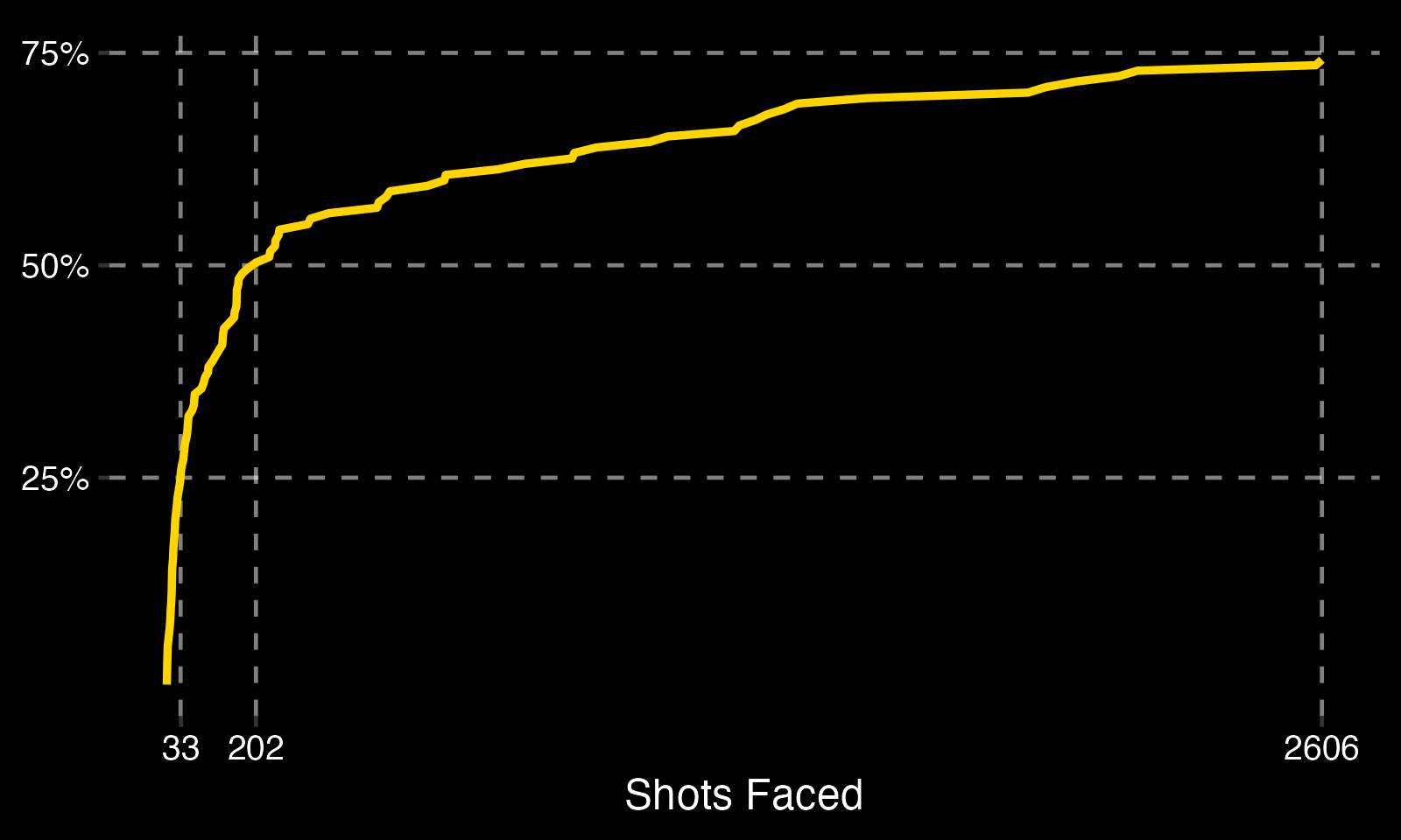
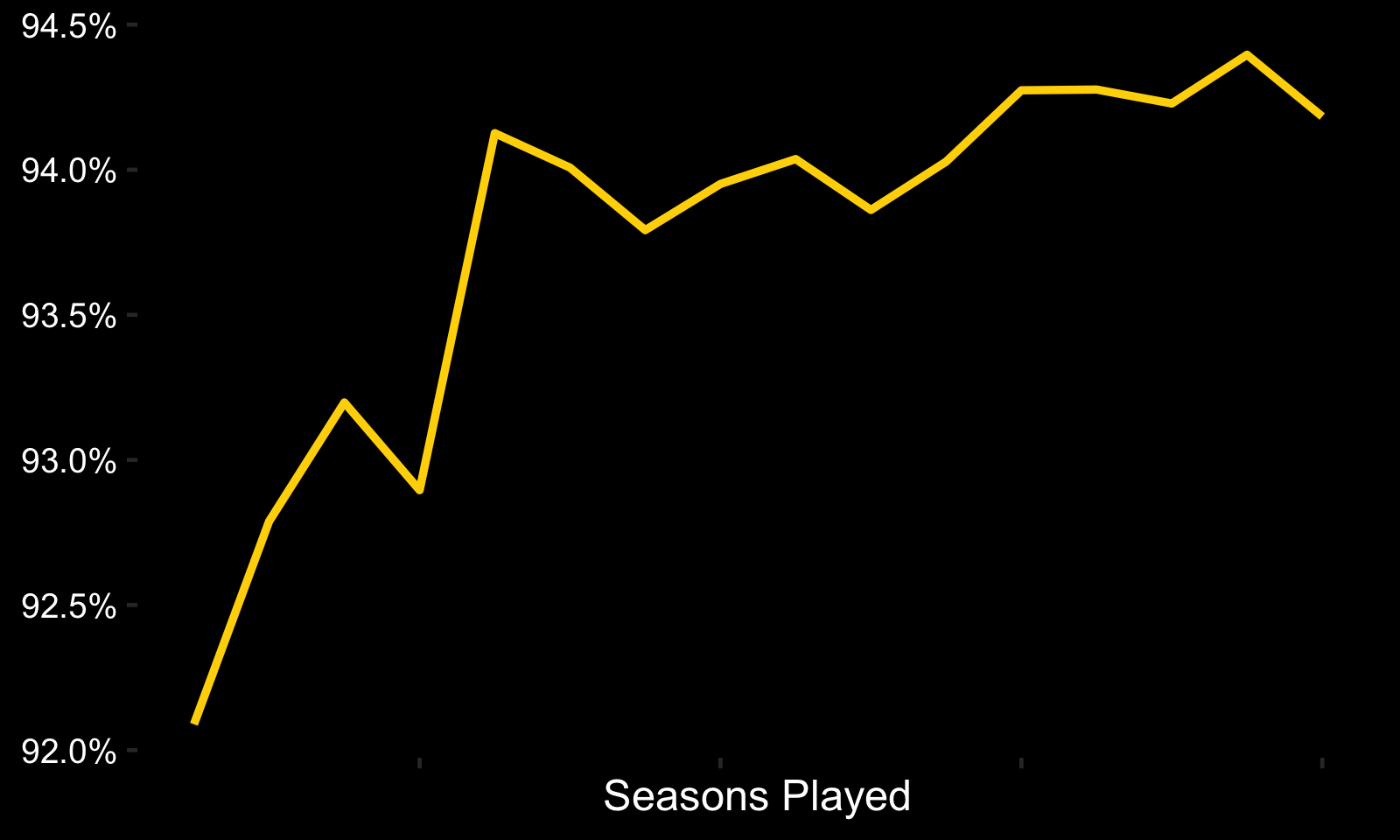
This is a problem. One possible solution to this was proposed by David Robinson in his Baysian series on baseball. Instead of fitting a beta distribution to batting averages, he fit a negative binomial distribution using 1) at bats and 2) hits. This can easily be applied to goalies using 1) shots faced and 2) adjusted saves. It has its problems, though (which, of course, David addresses in a string of fantastic blog posts, eventually turning into a book). The main problem is that it introduces bias - goalies who perform well are likely to get more opportunities to play compared to those who perform poorly. As proof, here's a plot showing the average AdjSV% by career seasons played:

Because of this bias, we're faced with a compromise: Do we weigh the observations by shots faced, which will lean the analysis towards better performing goalies, or do we treat all goalie careers equally, losing nearly 30% of our population (albeit less than 1% of shots faced) at the same time? Or... is there an alternative?

David's alternative was to fit a beta-binomial regression of batting averages on at-bats. Essentially, each at-bat total has its own prior. Though this is a good idea for his use case, it isn't great for mine. The problem is that I want to build a decision making tool for goalies who are still playing, and we don't know how many shots they will face in the future! This is the point of departure.

Combining Priors

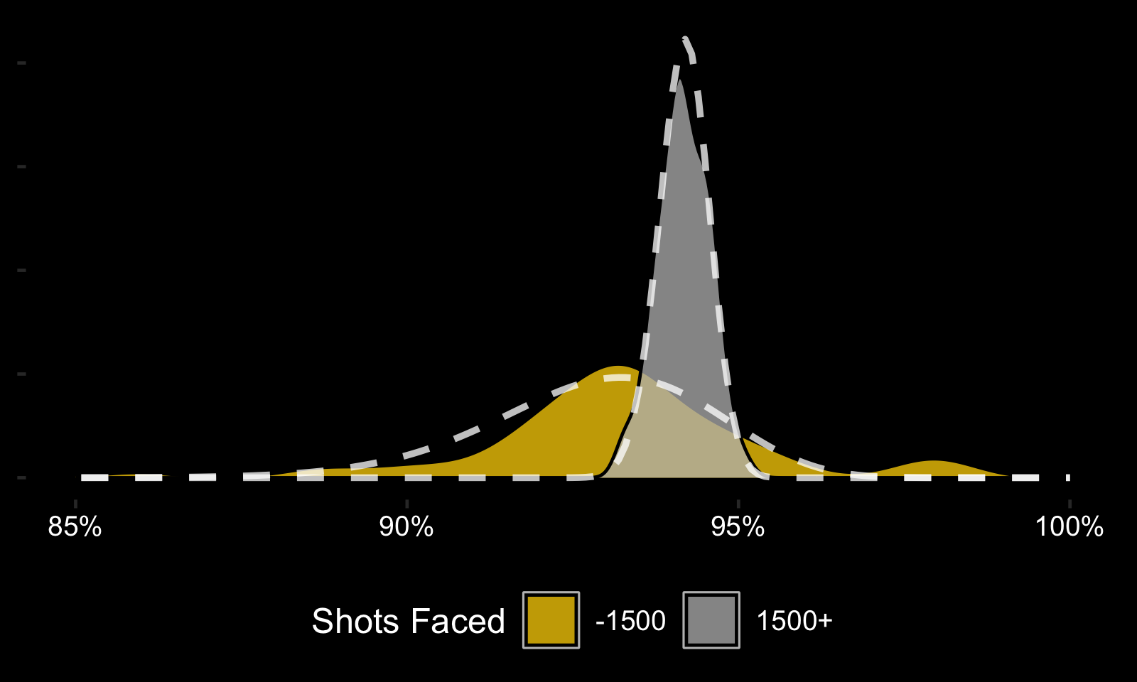
To address these issues, the Bayesian framework can be expanded to include two priors, glued together by a probability. The goalie career AdjSV% density plots are revisited, this time splitting goalies into two groups: those facing -1,500 shots and those facing 1,500+. From these group distributions, two separate priors can be built, and they can be merged by including a probability of a goalie belonging to each group, which can change as they face more shots. </p>

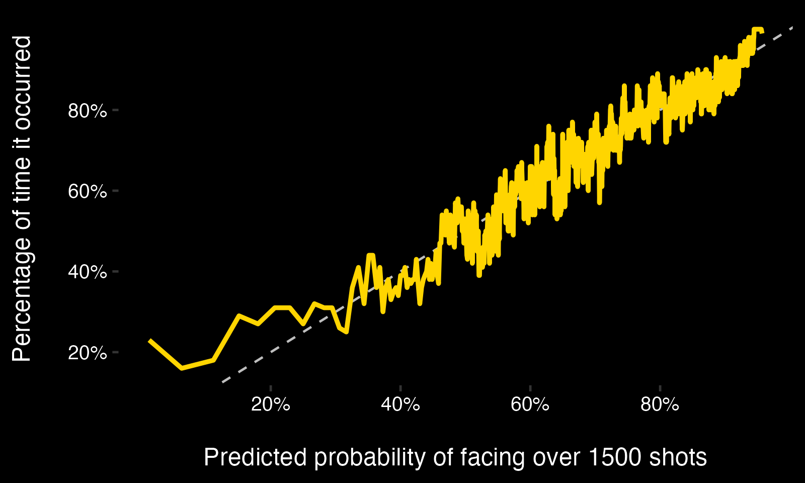
Here's a simple idea for the class probability described above: run a logistic regression using cumulative shots faced and AdjSV% onto the outcome of whether a goalie ended up facing 1,500+ shots. This model would be easy to train and interpret.

And, it turns out, such a model is well-calibrated:

The new equation to derive the posterior save percentage then becomes: P(1500+)*(alphaO + AdjSV%)/(alphaO + betaO + S) + P(-1500)*(alphaU + AdjSV%)/(alphaU + betaU + S) where: - P(1500+) = Predicted probability that goalie faces 1500+ shots in career. - alphaO = alpha from fitted beta distribution on goalies facing 1500+ shots. - betaO = beta from fitted beta distribution on goalies facing 1500+ shots. - P(-1500) = Predicted probability that goalie faces -1500 shots in career. - alphaU = alpha from fitted beta distribution on goalies facing -1500 shots. - betaU = beta from fitted beta distribution on goalies facing -1500 shots.

Code available here: https://github.com/spazznolo/goalie-performance/blob/main/posts/post-4.R