Assigning pick probabilities from user mock drafts
If you’re picking first at the next NHL draft, you want Lafreniere. If you’re picking second or third, you want Byfield or Stutzle. If you’re picking fourth, or fifth, or sixth, or seventh, you’re picking Rossi or Perffeti, or Raymond, or Drysdale… Notice how the list lengthens as you make your way through the draft? That’s because the uncertainty of a player being better than all other available players increases the deeper you get into the draft. So maybe you really like Rossi, but you’re picking sixth, and you want to be reasonably certain he will still be available. Well, what are the odds Rossi is still available at six? It’s hard to say.
Let’s say we only have our own rankings to go on. Instead of only predicting each player’s draft position, we could create probabilities of each prospect being drafted at each pick. Let’s use Rossi again as an example. Here’s how we might place probabilities on Rossi’s draft result:
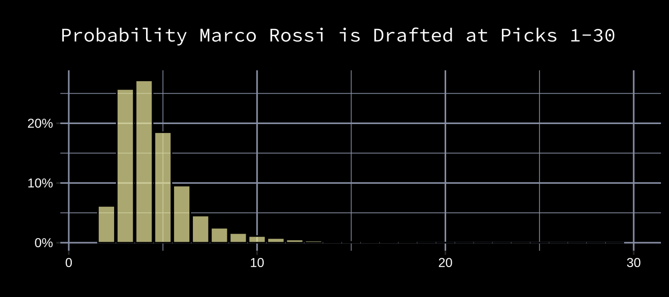
This is a probability distribution of Rossi’s predicted draft result. Though this is a step in the right direction, these are only our predictions of where Rossi might go. What if the teams drafting ahead of us don't rank him as highly? Their probability distribution for Rossi might look like this:
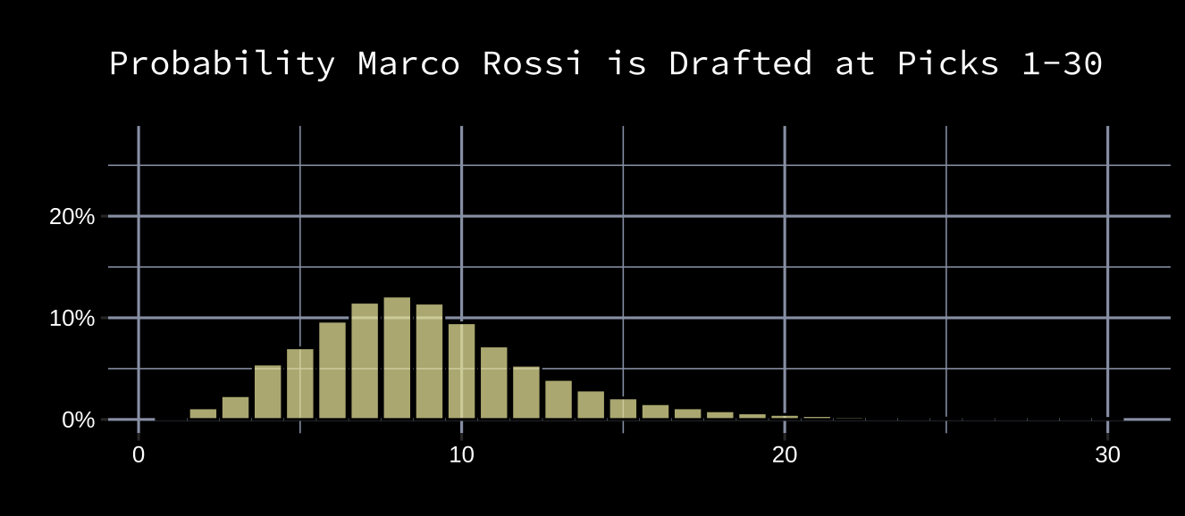
If the teams ahead of us view Rossi closer to the plot above, then he’ll likely slide lower than we predicted he would, and our chances of drafting him are higher than we previously thought. In fact, if we knew what other teams thought of him, we could pretty accurately predict where he’ll still be available in the draft, which allows us to either a) be comfortable we have a strong chance of picking him without trading up, or b) slide down a couple spots, pick up a mid-round pick and still get him. An important thing to remember is that Rossi’s draft position is much less affected by how we think of him than it is by how everyone else thinks of him.
In practice, no team will ever know exactly how every other team has ranked each prospect. Instead, player-pick probability distributions need to be approximated by other means. Dawson Sprigings outlined one way of doing this for Hockey-Graphs which used bayesian inference and pro rankings publishers. I’m going to outline another possible way, which uses mock drafts generated by users on Draft Site to derive probability density functions for each player.
An Example
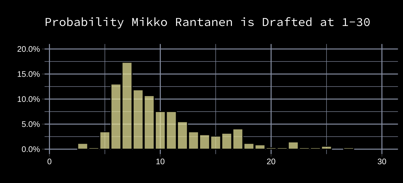
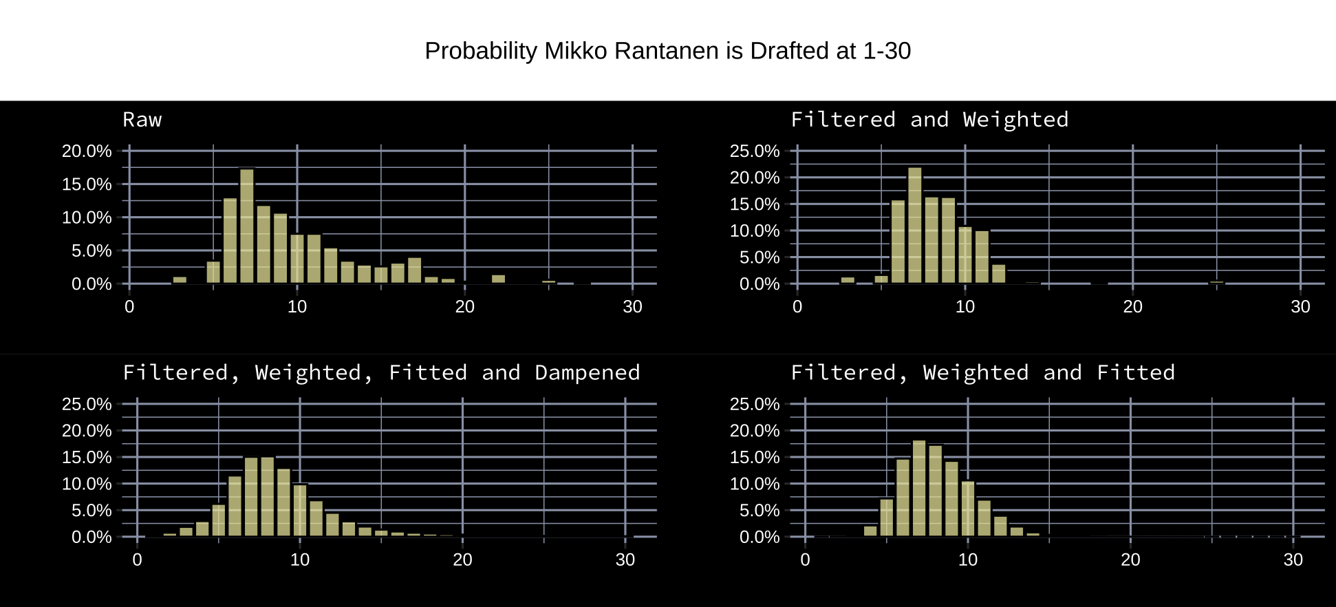
Draft Site, gets hundreds of user mock drafts each year. These mock drafts naturally create probability distributions for each player’s potential pick placement. For example, here was Mikko Rantanen’s in 2015 where each user’s draft was weighted equally.
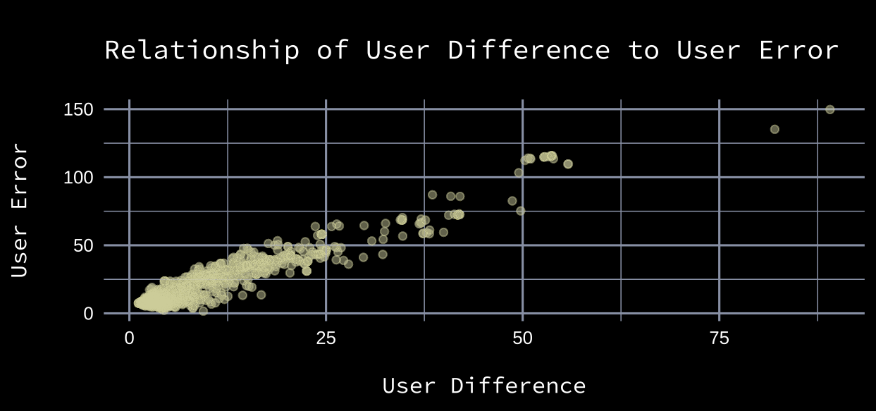
This distribution should be smoothed, but first, I'd like to address the fact that some mock drafts are more informative than others. A user who can more correctly predict a draft’s order is more valuable than one who cannot. Therefore, larger weights should be given to users who are likely more accurate in their mock draft. Thankfully, there are a couple quality indicators available: a user’s difference to the average user draft, and the number of days before the draft date that a user last updated their mock draft.
Mock Draft Quality Indicators
Difference to the Average Draft
Mikko Rantanen’s median pick from the raw user data was 9. If a user selected him 25th, they would be 16 spots off. A user’s absolute error rate can be computed for each pick in their mock draft. Below is the relationship of users’ mean absolute pick difference and their mean absolute pick error to the actual draft from 2015-2019. There’s a strong relationship between the two.
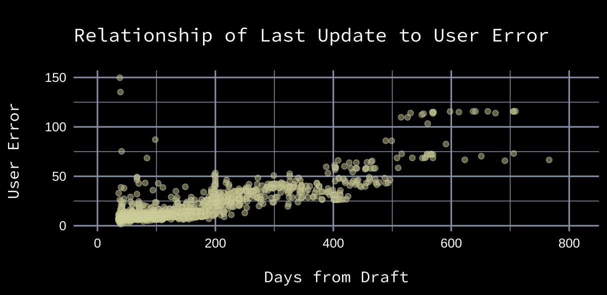
Days to the Draft
Usually, ranking publications will release a preliminary rankings list about a year before the draft. Then, as the draft approaches and player’s develop – or don’t - the rankings are updated. The plot below demonstrates that user data becomes more accurate as draft day approaches.
The variables discussed above were used to (1) filter what are likely low quality drafts and (2) create weights for each user mock draft. Players’ adjusted pick probabilities were then fit and dampened (more information on these decisions is available in the Notes section).
Comparing Probability Distributions
The Effect of Treatments on Player-Pick Probability Distributions
Here’s a visualization of the effects various treatments have on the user rankings.
The downside to user mock drafts is that prospect ranking is likely a hobby for most users. They may mostly rely on second hand information provided by hockey sites, experts, and prospect ranking models. Before going further, it’s important to measure its capacity for prediction. One way of doing this is to build a draft ranking from the data, and then measure its accuracy against professional ranking publishers.
Derived User Rankings vs the Pros
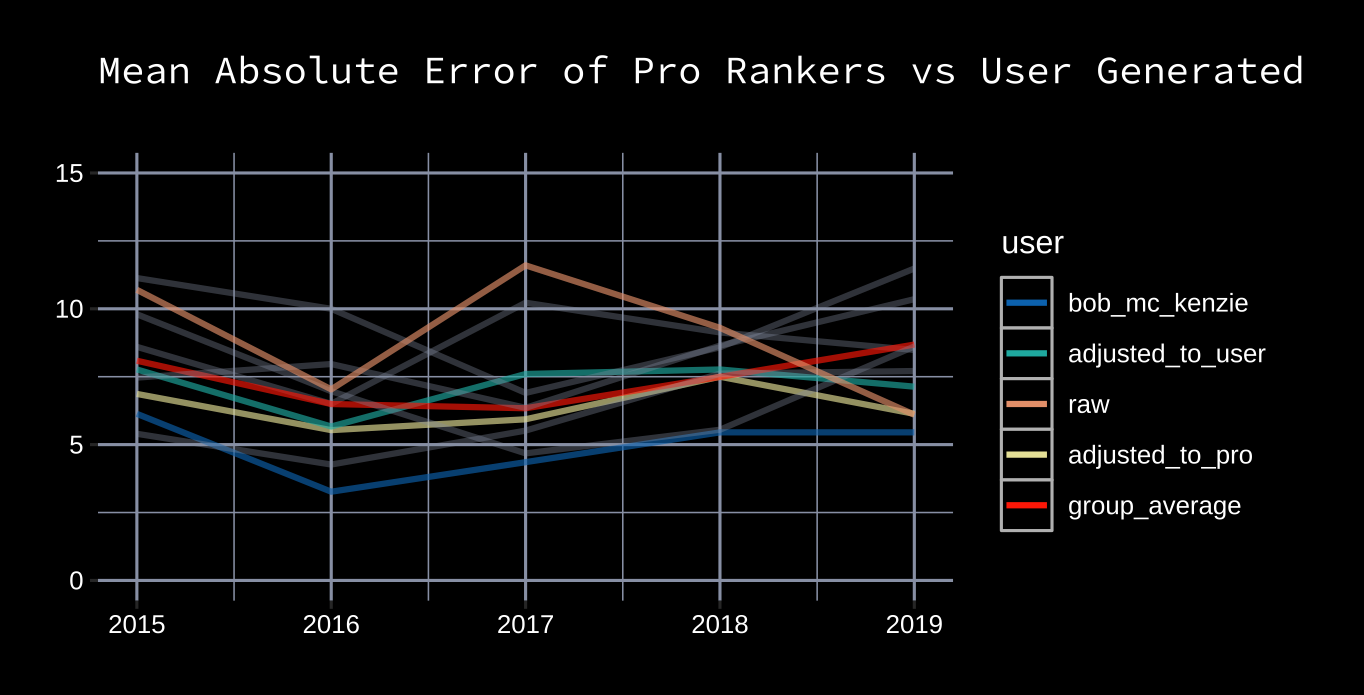
Draft rankings are derived from player-pick probability distributions by iterating through each pick of each draft, and drafting the player with the highest probability of being taken. After each pick, the player distributions are re-approximated (more information is available in the Analysis Notes section).Here is the mean absolute error of derived user draft rankings from 2015-2019 compared to various pro projections. All experts but Bobby Mackenzie, the gold standard of draft projections, have been greyed out. It's worth noting that the goal of some professional draft analysts is to predict which players will have the best careers, and not necessarily the order they might be picked. Purple is the group average.
User data, when properly treated, is competitive with pro ranking publications at predicting draft order. The advantage is that user data has built-in player-pick distributions which can be used to answer important questions about the draft.
Another Perspective on Probability Distributions
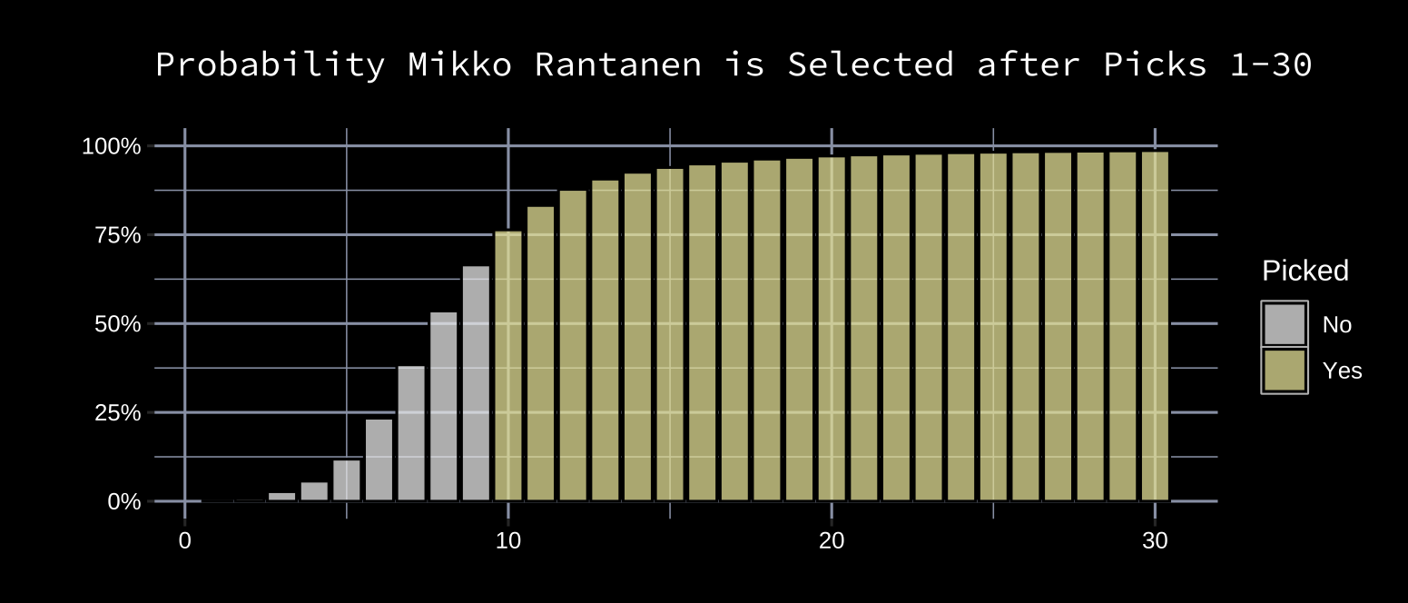
Here’s the probability Mikko Rantanen had of being selected at specific picks: 1, 0.1%; 2, 1.0%; 3, 2.6%; 4, 4.6%; 5, 7.9%. Another way to look at this is to say the probability Mikko Rantanen would be selected in the first five picks was 16.3% (the addition of each pick probability for picks 1-5). These cumulative probabilities can be calculated for each pick. Here’s what this looks like on a plot.
This is called a cumulative distribution (each pick takes the cumulative sum of all previous pick-probabilities). A pick-probability curve like the one visualized above can be derived for each player. Given that these cumulative pick-probabilities are the cornerstone of the analysis, it’s important to measure their accuracy. The fit of these curves can be evaluated by going through each pick and asking the questions: what was the probability of this player being drafted by this pick and was he drafted by this pick?
Evaluating the Fit
Either a player was drafted by a certain pick, or they weren’t. This is called a binary event, with values 0 (he wasn’t) and 1 (he was). Mikko Rantanen had a 55.5% probability of being drafted by the eighth pick, and the result was that he wasn’t yet picked (0). The error for the probability attributed to this event can be seen as 0.555-0 = 0.555. Rantanen also had an 86.4% probability of being drafted by the twelfth pick, and the result was that he was picked (1). The error for the probability attributed to this event can be seen as 0.864-1 = -0.136.Each player has probabilities attached for the first thirty picks of the draft. This is roughly 7,000 events. Errors can be attributed for these events the same way as they were outlined in the previous paragraph. Since the aim is to build well calibrated probability distributions, the brier score will be used to evaluate the fit. The calibration plot is plotted below along with Brier scores.
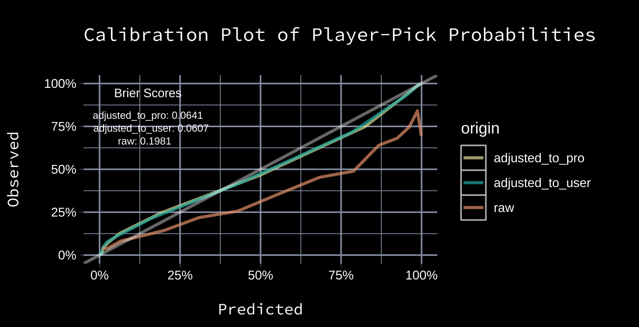
The perfect fit is the grey line, where outcomes occur the predicted percentage of time. Whenever a curve slides away underneath the line of perfect fit, like it does with the raw user data (and to a lesser extent the adjusted user data), it means the method tends to be overconfident in its assignment of probabilities. The plot above, along with the Brier scores, suggest the adjusted user data (score ~ 0.0604) is a better fit than raw user data (score ~ 0.198).
Cumulative player-pick probabilities for the 2020 draft are available here.
Notes
Filtering Users
Adjusted to User Average: 1. RMSE to user average < 15 2. Days to draft < 150Adjusted to Pro Consensus: 1. RMSE to pro consensus < 15 2. Days to draft < 150
Attributing Weights to Users
A linear regression is fit using: RMSE to user average, days to draft, (and RMSE to pro consensus for data weighted to pro consensus) as predictors and the RMSE to actual draft order as target. User weights are the inverse of the linear model predicted RMSE of user ranking to the actual draft order.Fitting Player Distributions
A gamma distribution is fit to adjusted data.Dampening Player Distributions
Player distributions are dampened by the variance observed in prior years. This is superior to the variance in the raw data because, in this case, it is caused by actual deviations as opposed to what are likely bad user predicitons.I wrote a similar article for the NBA Draft at Nylon Calculus.