flowchart TB
  rankings["PARTIAL PUBLIC RANKINGS"] --> complete["completed rankings"]
  time["TIME WEIGHTS"] --> weighted["weighted rankings"]
  publication["PUBLICATION WEIGHTS"] --> weighted
  complete --> weighted
  weighted --> strengths["Plackett–Luce strengths"]
  strengths --> drafts["simulated draft orders"]
  drafts --> probabilities["pick probabilities"]
  probabilities --> pickvalue["pick value"]
  team["TEAM PROSPECT VALUES"] --> pickvalue
  pickvalue --> decision["draft decision"]

  class rankings,time,publication,team phase
NHL Pick Probability
Building a probability-based drafting strategy from public draft rankings.
10 min read
Purpose
A draft ranking tells a team who it prefers. It does not say whether that player will still be available at its next pick. That distinction matters because a prospect’s draft position is much less affected by how one team thinks of him than by how everyone else does.
If a team likes a prospect but picks sixth, what are the odds he is still available? Could the team slide down, pick up another asset and still get him? It is hard to say from a ranking alone.
Historical pick-value charts describe the average return at each draft position. They are useful as a market reference, but drafts are not average: there are strong classes, weak classes, clusters of similarly talented players and sudden drops in value. A class-specific estimate preserves that shape.
Point estimates also hide uncertainty in prospect value. One of the main questions for teams picking between second and seventh in 2023 was whether to draft Matvei Michkov. He had signed a three-year contract in Russia. He met with only a few teams. He might have been the most talented player in the draft. He might never come to North America. Was it worth drafting that uncertainty when more reliable, though perhaps less skilled, players were available? Unless the uncertainty is included in the calculation, the decision is mostly left to instinct.
System
In practice, no team knows exactly how every other team ranks each prospect. Pick probabilities have to be approximated by other means. This system estimates pick probabilities by first fitting a rank-ordered model on public prospect rankings, and then simulating the draft from these latent player strengths. Then, these probabilities can be combined with a team’s own prospect values to create their personalized pick value chart.
Contents
Data
There are thousands of draft-eligible prospects. No publication can rank all of them, so every list is a partial ranking. This model restricts the population to prospects ranked in the top 100 by at least one publication. Each observation consists of a publication, its date, and a prospect’s rank. The decision stage requires one separate input, \(v_i\): the team’s own value for each prospect.
Parameters
Estimated from public rankings
| \(w_i\) | = | positive draft strength for prospect \(i\) |
| \(\mathbf w\) | = | the strengths of all prospects in the modeled pool |
Ranking weights
| \(l\) | = | a published ranking |
| \(d_l\) | = | days between ranking \(l\) and the draft |
| \(s(l)\) | = | publication which produced ranking \(l\) |
| \(t(d_l)\) | = | time weight returned by the fitted days-to-draft curve |
| \(\hat e_s\) | = | expected historical error for publication \(s\) |
| \(\rho_s\) | = | normalized inverse-error weight for publication \(s\) |
| \(\omega_l\) | = | final weight assigned to ranking \(l\) |
Ranking completion
| \(c_i\) | = | number of published rankings containing prospect \(i\) |
Supplied by the team
| \(v_i\) | = | the team’s value for prospect \(i\) |
Quantities produced by simulation
| \(D_j\) | = | prospect selected at pick \(j\) |
| \(R_j\) | = | prospects remaining before pick \(j\) |
| \(B_j\) | = | highest-valued prospect available at pick \(j\) |
| \(V_j\) | = | expected value of pick \(j\) |
Model
Ranked choices
A Plackett–Luce model assigns each prospect a positive strength \(w_i\). For completed ranking \(l=(i_{l,1},\ldots,i_{l,N})\), the probability of observing that order is
\[ p(i_{l,1},\ldots,i_{l,N}\mid\mathbf w) = \prod_{k=1}^{N} \frac{w_{i_{l,k}}} {\sum_{h=k}^{N}w_{i_{l,h}}}. \]
At each pick (or, position), the selected prospect is compared with all undrafted players on the list. This learns relative strength.
Ranking weights
Lists become more accurate as the draft approaches, and some publications are more closely aligned with observed draft order than others.
The time-weight function \(t(d)\) is an empirical lookup curve, scaled so that a ranking published immediately before the draft receives weight 1:
\[ t_l=t(d_l), \qquad t(1)=1. \]
Publication reliability is the inverse of expected historical error, normalized to have mean 1 across publications \(\mathcal S\):
\[ \rho_s = \frac{1/\hat e_s} {\frac{1}{|\mathcal S|}\sum_{r\in\mathcal S}1/\hat e_r}. \]
For a publication with several updates, its time weights are normalized before being multiplied by its publication weight:
\[ \omega_l = \rho_{s(l)} \frac{t(d_l)}{\sum_{h:s(h)=s(l)}t(d_h)}. \]
The denominator divides a publication’s influence across all of its lists. A publication represented by only one list instead receives \(\omega_l=\rho_{s(l)}t(d_l)\).
Likelihood
For \(L\) completed rankings, the fitted strengths maximize the weighted log-likelihood
\[ \hat{\mathbf w} = \underset{\mathbf w}{\arg\max} \sum_{l=1}^{L} \omega_l \log p(i_{l,1},\ldots,i_{l,N}\mid\mathbf w). \]
Pick probability
The same probability rule is then run forward to simulate a draft. If \(R_j\) is the set of prospects remaining before pick \(j\), then
\[ P(D_j=i\mid R_j,\hat{\mathbf w}) = \frac{\hat w_i} {\sum_{h\in R_j}\hat w_h}, \qquad i\in R_j. \]
The selected prospect is removed from \(R_j\), and the draw is repeated for the next pick. Simulation is therefore the fitted ranking model run forward, not a separate probability model.
Pick value
Counting how often player \(i\) is still undrafted before pick \(j\) estimates
\[ P(i\text{ is available at pick }j). \]
Availability probabilities overlap: Michkov and Carlsson can both be available at pick four. To value a pick, the probabilities must instead describe which player is the best available option. Let \(B_j=i\) mean prospect \(i\) is the highest-valued player remaining at pick \(j\). Then
\[ V_j=\sum_i P(B_j=i)\,v_i, \]
where \(v_i\) is the team’s value for prospect \(i\).
Draft Optimisation
The usual advice is to take the best player available. The better rule is to take the best player available only when the risk of losing him before the next pick is greater than the value gained by selecting somebody else first.
For current pick \(j\), next pick \(k\), remaining prospect set \(R_j\), and prospect value \(v(a)\), the two-pick decision can be written as
\[ a^* = \underset{a\in R_j}{\arg\max} \left[ v(a) + \operatorname E\!\left\{ \max_{b\in R_k(a)}v(b) \right\} \right]. \]
\(R_k(a)\) is the random set of prospects still available at the next pick after selecting \(a\) now. The first term rewards the current selection; the second preserves the option value of the next pick.
Estimation
Completing partial rankings
The model first makes the partial rankings complete. After restricting the pool to prospects who appear in at least one top 100, it counts how many rankings contain each prospect. For the unranked tail of a list, missing prospects are drawn without replacement using those appearance counts, \(c_i\), as weights.
This makes the rankings usable, but not truly complete. A prospect outside the modeled pool receives no chance of being selected. The problem grows as the draft continues, so the probabilities are most useful near the top and become less reliable in later rounds.
Fitting prospect strengths
The time weights come from the earlier mock-draft work. For each mock, error to the eventual draft order was compared with the number of days remaining before the draft; a LOESS curve smoothed that relationship into a daily weight. Using draft day as the index, a ranking published one month out receives roughly 90% weight; two months, 77%; four months, 50%; and one year, 17%.
Publication weights are estimated from rankings released between 2018 and 2022. Each publication’s error is calculated against the eventual top 30, with mistakes near the top carrying more weight. Performance in the other available years is used to estimate its expected error, then the inverse of that error becomes its reliability weight. The weights are normalized to average one; a publication with no history receives 0.75.
The final ranking weights combine time and publication reliability as shown above. The Plackett–Luce fit also adds a hypothetical reference prospect. Every real prospect weakly beats and loses to that reference through pseudo-comparisons with weight 0.05. This connects parts of the comparison network which otherwise do not meet and lightly pulls poorly connected prospects toward equal strength.
This treatment deliberately flattens time. A late ranking counts more than an early one, but prospect strength does not evolve inside the model. Rankings change because prospects and scouts do things between publications, not because time itself passes.
A Bayesian version was also explored, adapted from Tyrel Stokes’s work on rank-ordered events, with weights representing tier importance and ranking noise. The results below use the time-weighted frequentist fit.
Simulating draft order
The fitted strengths define a distribution over draft order. One hundred thousand drafts are generated by drawing prospects without replacement, using the fitted strengths as weights. Counting the simulated orders produces a probability that each prospect is selected at—or remains available for—each pick.
The implementation is available in the draft-rankings repository.
Applications
Montreal: pick value
The 2023 Canadiens picked fifth, just outside a consensus top group of Connor Bedard, Adam Fantilli, Matvei Michkov and Leo Carlsson. Should they trade up to guarantee one of them, or take the risk that somebody slides? The more interesting question is: what information are they using to even make that decision?
Suppose Montreal values the top prospects as follows.
| Prospect | Seven-year value |
|---|---|
| Connor Bedard | 24 WAR |
| Adam Fantilli | 19 WAR |
| Matvei Michkov | 17 WAR |
| Leo Carlsson | 14 WAR |
| William Smith | 10 WAR |
The model estimates the chance that each player remains available at each pick.
| Pick | Bedard | Fantilli | Michkov | Carlsson | Smith |
|---|---|---|---|---|---|
| 1 | 100% | 100% | 100% | 100% | 100% |
| 2 | 0.2% | 99.8% | 99.9% | 99.9% | 100% |
| 3 | 0.0% | 21.0% | 88.1% | 93.7% | 99.4% |
| 4 | 0.0% | 2.8% | 42.0% | 69.1% | 97.0% |
| 5 | 0.0% | 0.2% | 11.1% | 26.9% | 91.9% |
Then, using the proposed draft optimisation equation, each pick is worth
| Pick | Proposed value |
|---|---|
| 1 | 24 WAR |
| 2 | 19 WAR |
| 3 | 17.8 WAR |
| 4 | 15.6 WAR |
| 5 | 11.9 WAR |
In this example, moving from pick five to pick four adds an expected 3.7 WAR. A trade creates value for Montreal only if the additional assets surrendered are worth less than that difference.
Montreal: prospect uncertainty
These values are still point estimates. Replacing them with distributions allows the same calculation to include prospect uncertainty. Instead of assigning Bedard exactly 24 WAR, suppose his seven-year value is normally distributed with mean 24 and standard deviation 3.
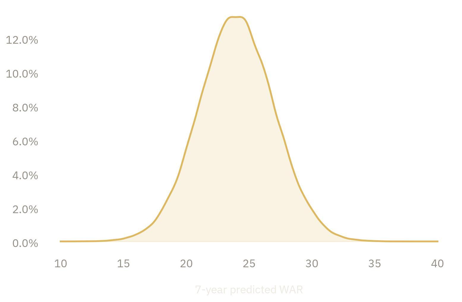
Under this illustrative distribution, Bedard has a 50% chance of providing roughly 22–26 WAR, a 25% chance of exceeding 26 WAR, and a 25% chance of falling below 22 WAR. The numbers are only an example; the point is that prospect value can be represented by a distribution rather than a single estimate.
The other prospects can be represented in the same way. Michkov receives the widest distribution, reflecting greater uncertainty about both his development and whether his value will be realized in the NHL.
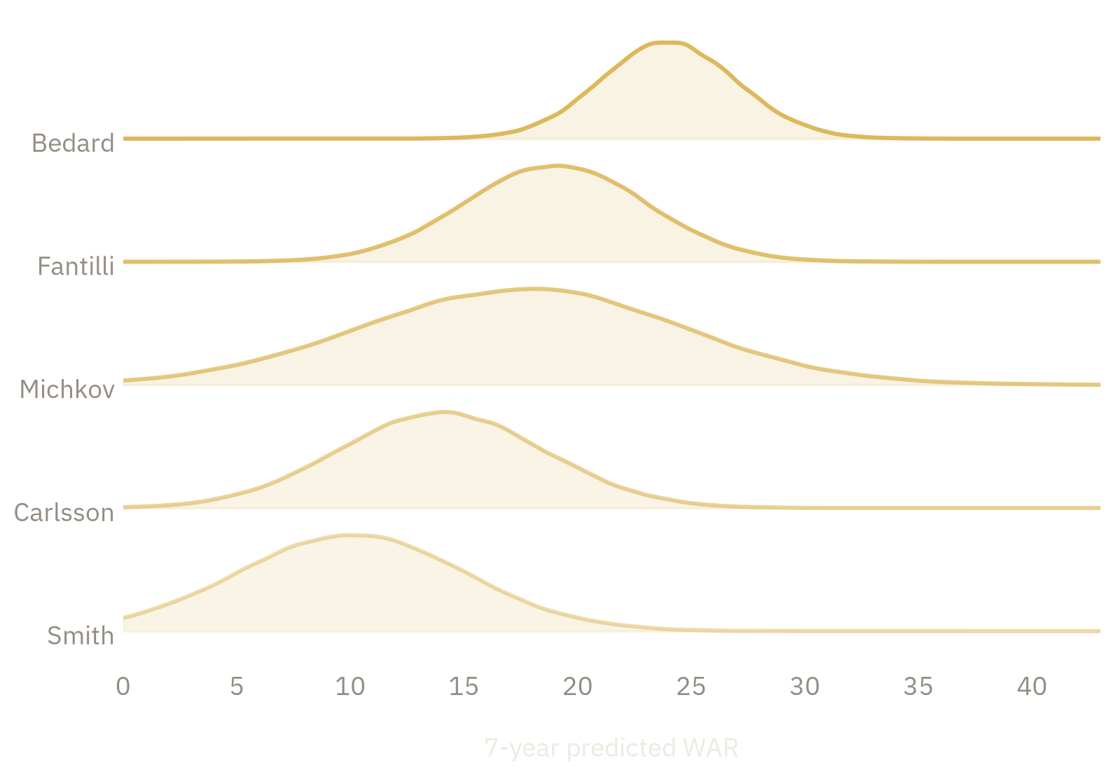
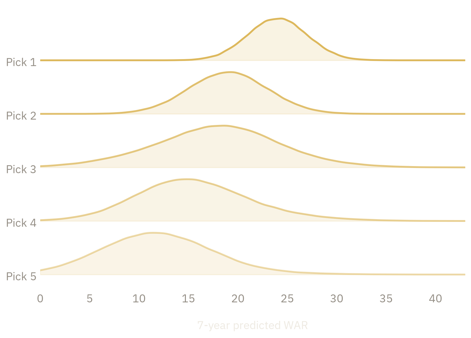
Sampling a prospect value and a draft order together produces a distribution for the value of every pick.
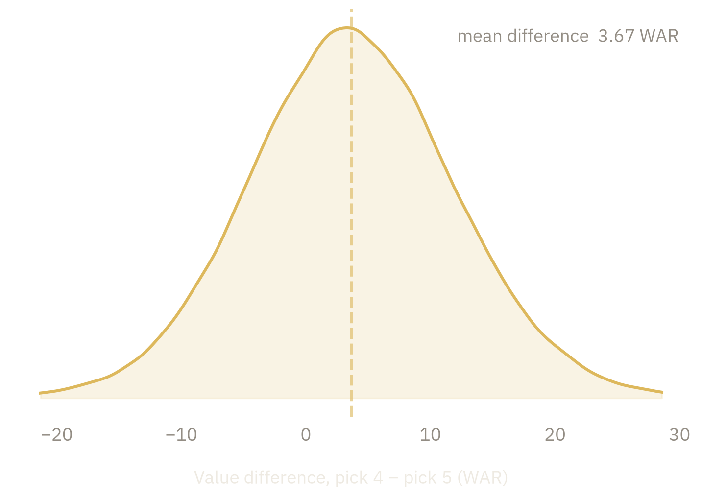
The distribution of the difference answers the trade question directly. Under these assumptions, pick four is worth more than pick five in 67.3% of simulations, with a mean difference of 3.7 WAR.
Detroit: drafting strategy
The 2023 Red Wings held picks 9 and 17. The example below combines pick probabilities with three public boards and a historical prospect-value curve. The question is not simply who each board ranks highest at nine, but which choice produces the greatest expected value across both picks.
| Board | Choice at 9 | Value at 9 | Value at 17 | Total value |
|---|---|---|---|---|
| Peters: best player available | Matthew Wood | 7.1 | 5.8 | 12.9 |
| Peters: optimal choice | Zach Benson | 6.7 | 6.8 | 13.5 |
| McKenzie: optimal choice | Dalibor Dvorsky | 7.1 | 5.9 | 13.0 |
| Robinson: optimal choice | Zach Benson | 8.2 | 5.9 | 14.2 |
McKenzie and Robinson should take their best player available. Peters should defer on Matthew Wood and select Zach Benson: the immediate loss in value is smaller than the expected gain at pick 17.
Validation
For each prospect and pick, the model produces the cumulative probability that the prospect has already been selected. After the draft, this can be compared with the observed result: selected by that pick or not selected by that pick.
Across the first 64 picks, the probabilities were generally well calibrated. They were too certain in the top ten, where the model placed too much probability on a narrow group of outcomes. One draft is not enough to precisely estimate calibration, but it identifies the main weakness in the current probabilities.
As a result, the sportsbooks cooked us.