Goalie Performance
13 min read
This article consolidates five posts published between 2023 and 2024.
EMPIRICAL BAYES
Goaltenders make up the least predictable position in hockey. Their behavior confounds analysts and casual fans alike. It isn’t uncommon for a good goalie to have a below replacement level year, or for an unknown goalie to come in and dominate the league for a stretch of time. This may partly explain the relative dearth of analysis on goalies - they’re voodoo, it’s often said.
This analysis estimates goalie performance using an empirical Bayes framework. Similar applications were outlined in previous papers. The Bayesian framing lets us partially pool noisy goalie results towards a population distribution, quantify what remains uncertain, and make direct probability statements about the players. The idea is first sketched using raw save percentage, then refined.
The figures were rebuilt in Python from MoneyPuck’s current historical files for the original 2007–2022 window. Because historical expected-goal estimates can be revised, a few reconstructed values differ modestly from the figures published in 2023.
Throughout this first pass, I will distinguish a goalie’s observed Fenwick save percentage from their underlying Fenwick save probability, \(\theta_i\). The observed percentage describes what happened in a particular sample. \(\theta_i\) describes the rate we would expect over repeated, comparable attempts. We do not observe it exactly; we represent what we know about it with a distribution.
The empirical Bayes approach involves two steps: learn a prior from the population, then update it with the individual goalie’s results.
Learn from the population. Imagine that an unknown goalie emerges. What can we say about their underlying Fenwick save probability before they have faced a shot? Could it plausibly be .930, .940, or .950?
Fenwick save percentage is the proportion of unblocked shot attempts that do not become goals.1 To build a first population estimate, we can look at the career 5v5 Fenwick save percentages of goalies who faced at least 200 attempts. The cutoff suppresses the noisiest short careers, but it also introduces selection; I return to that problem later.
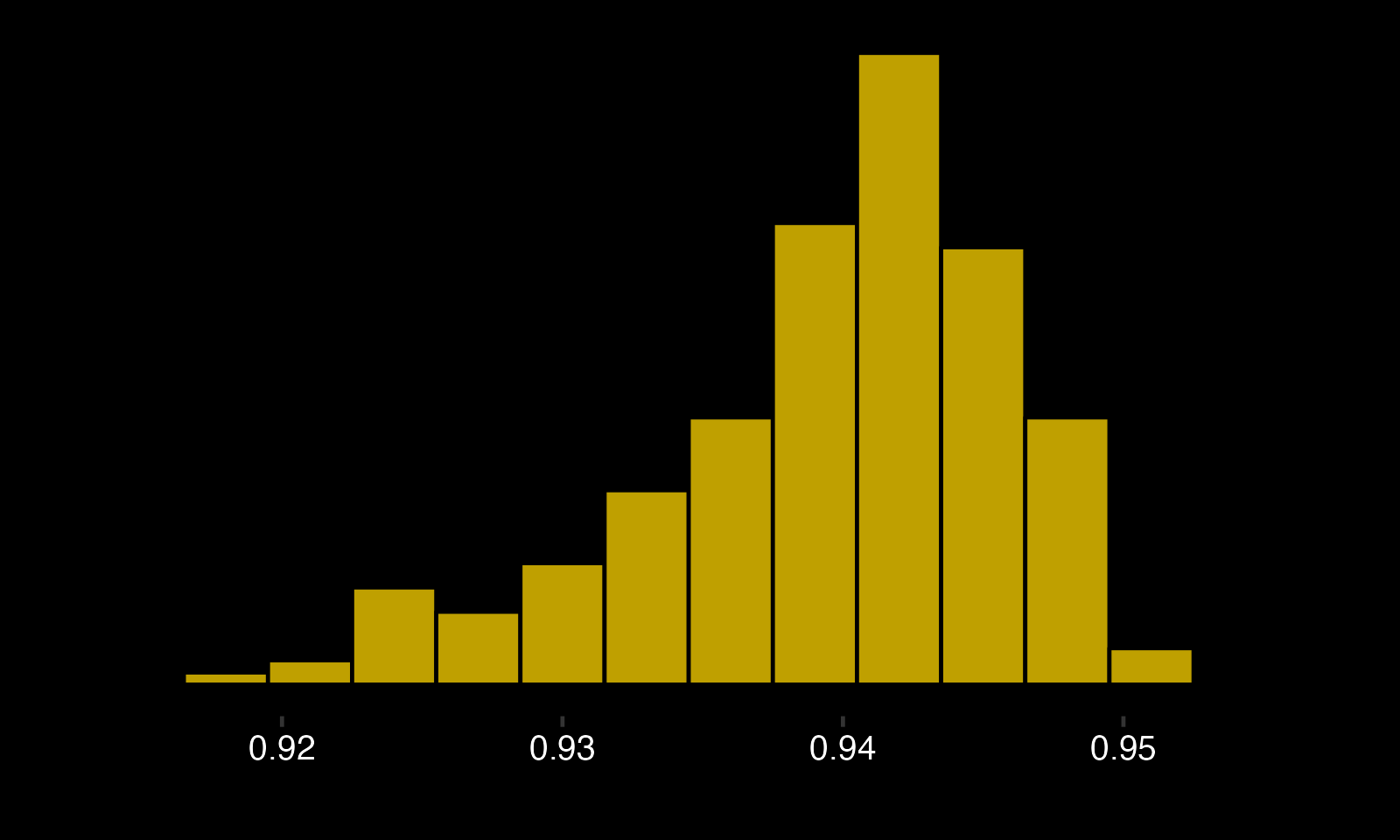
The histogram is a rough picture of the population, including sampling noise. Rather than treat every bump as meaningful, we fit a smooth distribution to it.
The beta distribution is a natural first prior for a probability: it is bounded between zero and one and is conjugate to the binomial likelihood. Fitting a beta distribution to the career Fenwick save percentage distribution yields the following result.
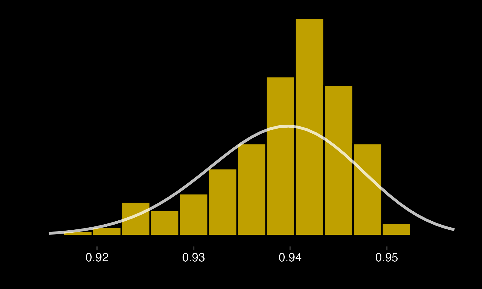
The fit is… not really good, but it serves its purpose as an introduction to the framework. More importantly, fitting a beta directly to career percentages treats rates based on different numbers of attempts as equally informative. A beta-binomial population model would handle those denominators more coherently. For now, the beta is a useful working approximation.
The beta distribution has two hyperparameters, \(\alpha\) and \(\beta\), which behave like prior non-goal and goal counts. Here, the fitted values are 852 and 55.6: before observing a particular goalie’s results, the model begins with information equivalent to 852 non-goal attempts and 55.6 goals. The prior mean is .9388, a little below the .9406 median among goalies who faced at least 200 attempts.
Update with the goalie. Let \(Y_i\) be a goalie’s non-goal outcomes across \(N_i\) unblocked attempts. The model is:
\[ \begin{aligned} \theta_i &\sim \operatorname{Beta}(\alpha,\beta), \\ Y_i \mid \theta_i &\sim \operatorname{Binomial}(N_i,\theta_i), \\ \boxed{\theta_i \mid Y_i} &\sim \operatorname{Beta}(\alpha + Y_i,\ \beta + N_i-Y_i). \end{aligned} \]
In plain language, we add the observed non-goals to \(\alpha\) and the observed goals—not all shots—to \(\beta\). When a goalie has faced only a few attempts, their estimate remains close to the population mean and their posterior remains wide. With more attempts, their own results carry more weight and the posterior narrows.
As an example, let’s plot the posterior distributions for two 24-year-old goalies: Jake Oettinger and Jeremy Swayman.
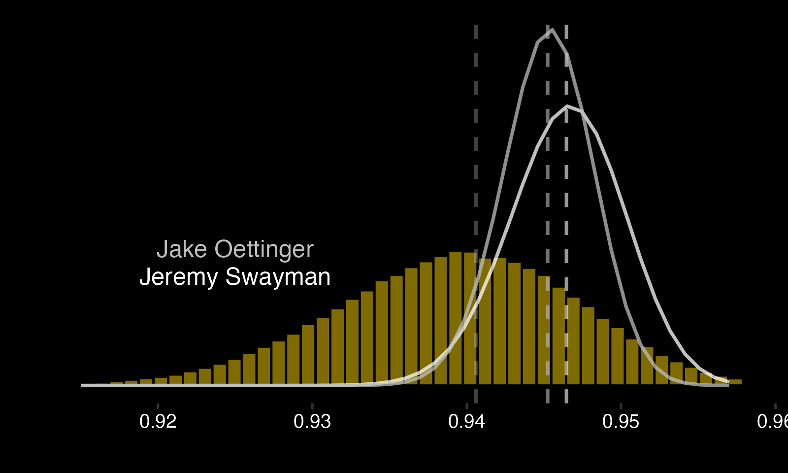
The reconstructed model gives Swayman a 66.2% probability of having the higher underlying Fenwick save probability. His probability of exceeding the .9406 population median is 93.8%, compared with 90.8% for Oettinger. Oettinger has faced more attempts, so his posterior is narrower even though its centre is slightly lower.
These probabilities are conditional on a deliberately simple model:
- Unblocked attempts are treated as comparable and conditionally independent.
- Each goalie’s underlying probability is treated as constant across their career.
- Shot quality, age, team context, and scoring environment are ignored.
- The population distribution is assumed to be beta.
- The fitted hyperparameters are treated as fixed, so their estimation uncertainty is not propagated.
- Goalies who faced fewer than 200 attempts are excluded, creating a selection problem.
These assumptions are intentionally strong. The rest of the analysis relaxes them one at a time.
ACCOUNTING FOR SHOT QUALITY
Not all attempts are equally difficult. Expected-goals models estimate that difficulty from the location and context of each attempt. MoneyPuck publishes one such estimate for every unblocked NHL attempt using a logistic regression model.
Shot-quality-adjusted performance is usually expressed as goals saved above expected. That is an intuitive counting statistic, but it is not a probability and can take any real value. To preserve the rate-scale framework above, I instead recenter the difference between observed and expected Fenwick save percentage around a common league benchmark.
Let \(G_i\) be observed goals, \(X_i\) expected goals, and \(N_i\) unblocked attempts for goalie \(i\). Let \(\mu_x\) be the mean season-level expected Fenwick save percentage in the sample; it serves only as a common reference point.
\[ \begin{aligned} \mathrm{FSV}_i &= 1 - \frac{G_i}{N_i}, \\ \mathrm{xFSV}_i &= 1 - \frac{X_i}{N_i}, \\ \boxed{\mathrm{AdjSV}_i} &= \mu_x + \left(\mathrm{FSV}_i-\mathrm{xFSV}_i\right). \end{aligned} \]
The quantity in parentheses is performance relative to the difficulty of the attempts faced. Adding \(\mu_x\) puts that difference back on a familiar save-percentage scale. A goalie who performs exactly as expected receives \(\mathrm{AdjSV}_i=\mu_x\).
There is an important approximation here. \(N_i\mathrm{AdjSV}_i\) is a fractional adjusted non-goal count, not a count of observed binary outcomes. Feeding it into the beta update preserves the useful shrinkage calculation, but the resulting model is no longer a literal beta-binomial data-generating process.
The distribution below shows career AdjSV% for goalies who faced at least 200 attempts, with fitted beta and Weibull curves.
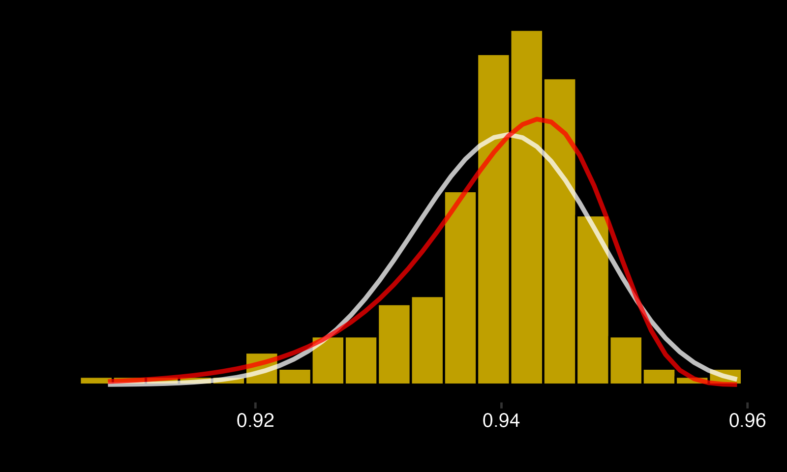
The Weibull follows this particular histogram more closely, but visual fit is not enough, and its support extends beyond one. I retain the beta as a bounded working prior. Its fitted parameters behave like 980 prior non-goal attempts and 63 prior goals, slightly more information than the raw-rate prior.
Let’s revisit the Jake Oettinger and Jeremy Swayman comparison.
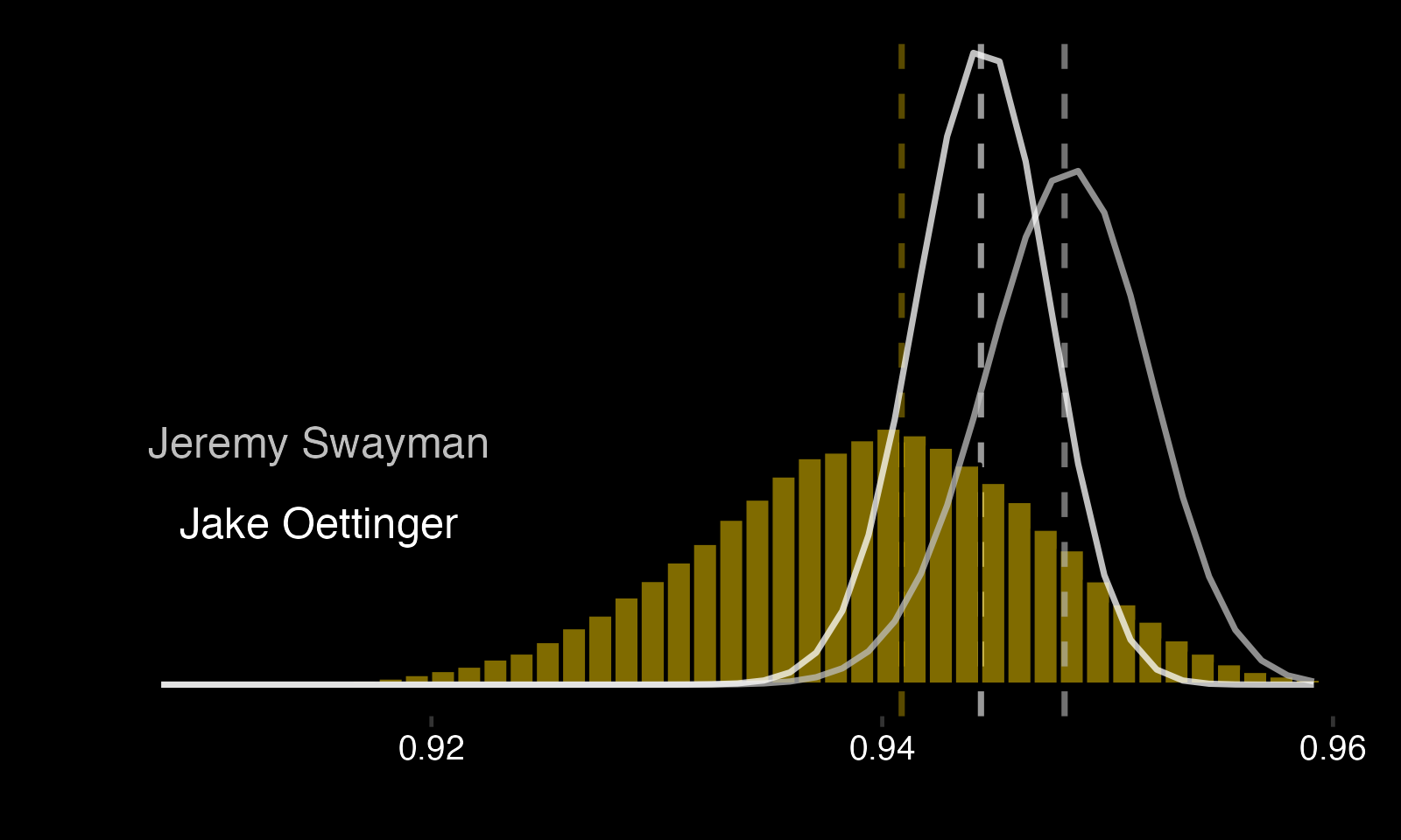
After accounting for attempt difficulty, the model gives Swayman an 83.4% probability of having the higher underlying adjusted rate, up from 66.2%. His probability of exceeding the median benchmark is 94.9%, compared with 70.7% for Oettinger. The mechanism is intuitive: Swayman’s xFSV% is 94.07%, compared with Oettinger’s 94.39%, meaning the model considers Swayman’s average workload more difficult.
Comparing the estimates
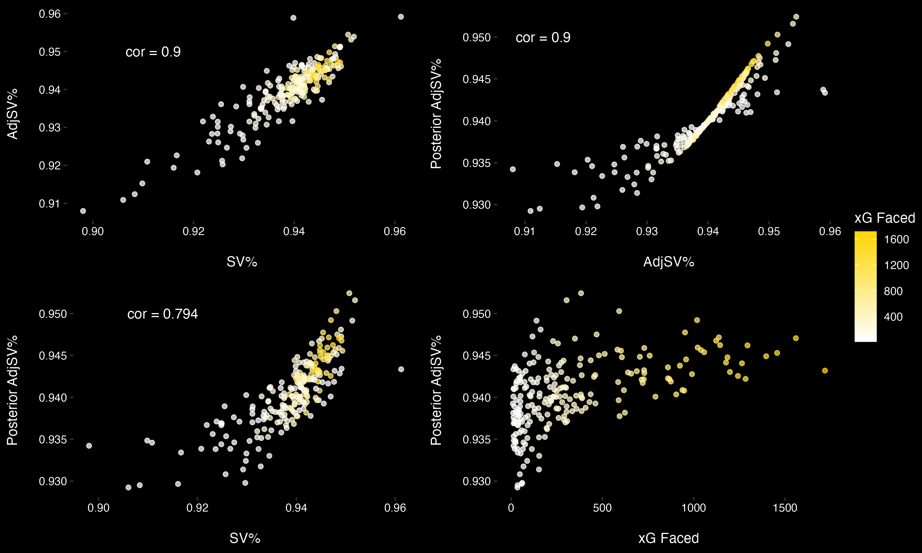
The four panels below separate the two operations being performed: adjusting for attempt difficulty and shrinking noisy estimates towards the population.
- Raw and adjusted save percentage remain strongly related (\(r=.921\)). Shot quality changes the estimate without discarding most of the signal in the observed rate.
- The adjusted and posterior-adjusted rates correlate at \(r=.899\), but the relationship bends around the prior mean. Small-workload estimates are pulled inward; large-workload estimates remain closer to the diagonal.
- Combining both operations lowers the correlation between raw and posterior-adjusted save percentage to \(r=.814\). Some goalies therefore move meaningfully once both context and uncertainty are included.
- The association between workload and posterior performance is partly a selection process: goalies who perform well tend to earn more opportunities. These plots cannot tell us that playing more causes improvement.
- The changing spread is expected when goalies have unequal sample sizes and receive different amounts of shrinkage. Calling it heteroskedasticity describes the shape, but not its cause.
The main result is modest but useful: shot quality changes whom we prefer, while partial pooling changes how certain we should be. The same figure also warns against interpreting career length as an independent measure of ability.
ADJUSTING FOR AGE
Goalie performance changes with age: players generally improve, reach a peak, and then decline. The timing and shape of that curve vary across published estimates, so I estimate one directly from the MoneyPuck sample.
- Obtain goalie birth dates.
- Derive goalie age for each game.
- Define new analysis population (we won’t find every goalie’s date of birth).
- Explore age.
- Adjust for age.
Finding goalie birth dates
I matched each goalie’s date of birth from MoneyPuck’s player lookup, supplementing gaps for retired players from the NHL player API. All 314 goalies in the reconstructed sample were linked.
Exploring age
I first group attempts by goalie age, rounded to one decimal place, and calculate the pooled save percentage within each age. Points are paler where fewer attempts were observed.
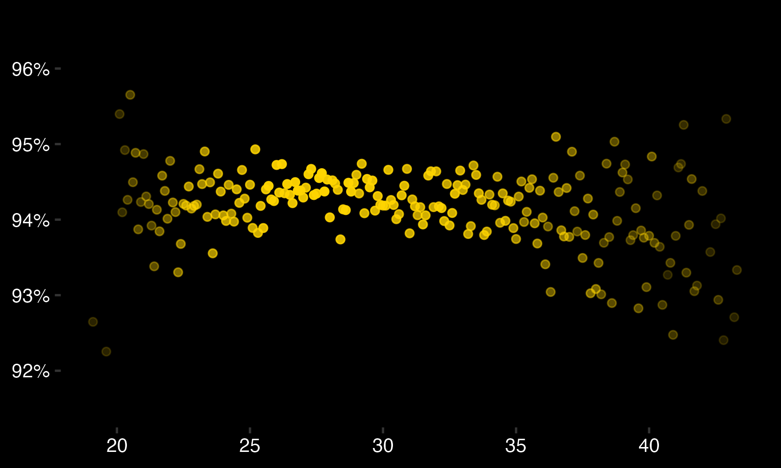
Most of the information lies between ages 23 and 35. There is a faint age pattern, but the cross-sectional curve mixes aging with selection: the goalies still playing at older ages are not comparable to everyone who entered the league.
To reduce that bias, I use the delta method described by Tango Tiger and applied in later hockey aging research. Rather than comparing different goalies at different ages, it compares each goalie’s performance with their own performance one year earlier.
Here are the steps:
- Calculate each goalie’s change in adjusted save percentage from one age to the next.
- Take the attempt-weighted arithmetic mean of those changes at each age.
- Remove sparsely represented ages below 22 and above 38.
- Accumulate the annual changes and normalize the curve to zero at its peak.
Altogether, this gives us the curve below:
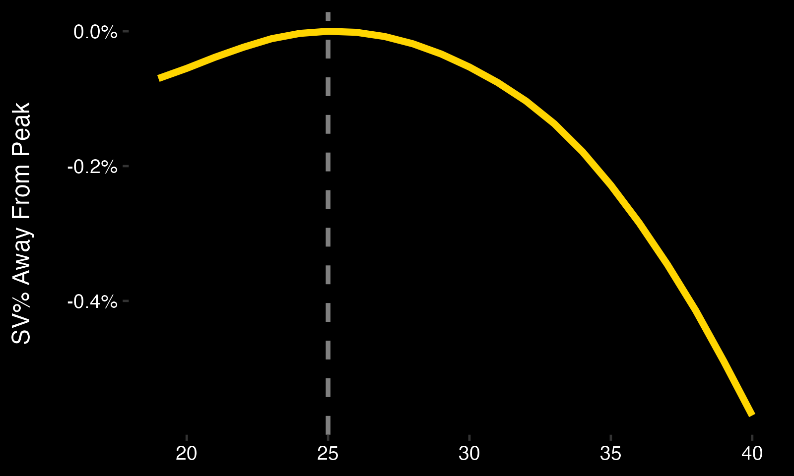
In the reconstructed sample, the fitted curve peaks around age 27. That lies between some previous work and later-peak estimates. It should be read as a descriptive adjustment, not a universal biological curve: weighting, survivor selection, and revisions to historical expected-goal values all influence its shape.
Applying the adjustment
I incorporate age through the same expected-rate term used for attempt difficulty. Let \(a(t)\geq0\) be the estimated performance gap between age \(t\) and the age-27 peak, with \(a(27)=0\). The age-adjusted expected rate is therefore \(\mathrm{xFSV}_i-a(t_i)\).
\[ \begin{aligned} \mathrm{xFSV}^{\mathrm{age}}_i &= \mathrm{xFSV}_i-a(t_i), \\ \boxed{\mathrm{AdjSV}^{\mathrm{age}}_i} &= \mu_x+\left(\mathrm{FSV}_i-\mathrm{xFSV}^{\mathrm{age}}_i\right) \\ &= \mu_x+\left(\mathrm{FSV}_i-\mathrm{xFSV}_i+a(t_i)\right). \end{aligned} \]
The adjustment therefore asks a narrower question than a raw age comparison: how far was this performance above or below expectation after accounting for both attempt difficulty and where the goalie sat on the estimated age curve? The answer remains conditional on the curve rather than a timeless property of the player.
CAREER LENGTH AND THE PRIOR
The 200-shot cutoff
The 200-attempt cutoff removes 91 of 314 goalies, or 29.0%. The career-attempt distribution shows how severe that filter is:
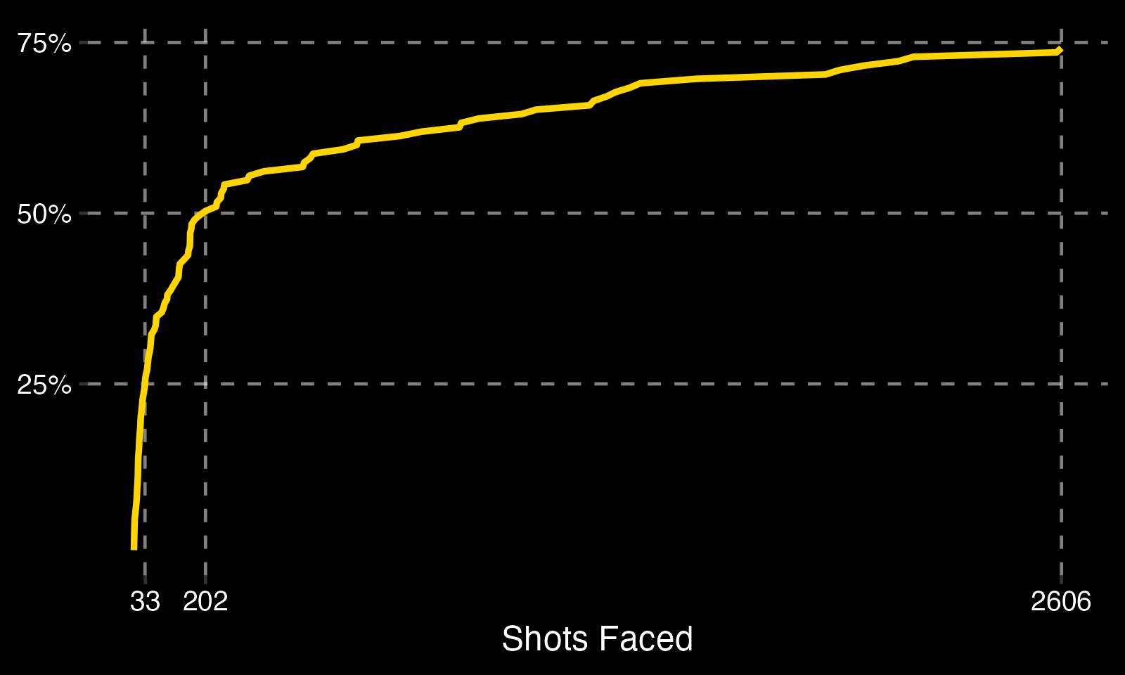
This matters because the excluded careers contain information, but not information of equal precision. Related empirical Bayes work by David Robinson models the observed rate and number of opportunities together. Hockey adds a complication: opportunity is endogenous. Goalies who perform well tend to receive more starts, so career length is partly an outcome of performance rather than an independent exposure.
The association is visible when average AdjSV% is plotted against career seasons played:
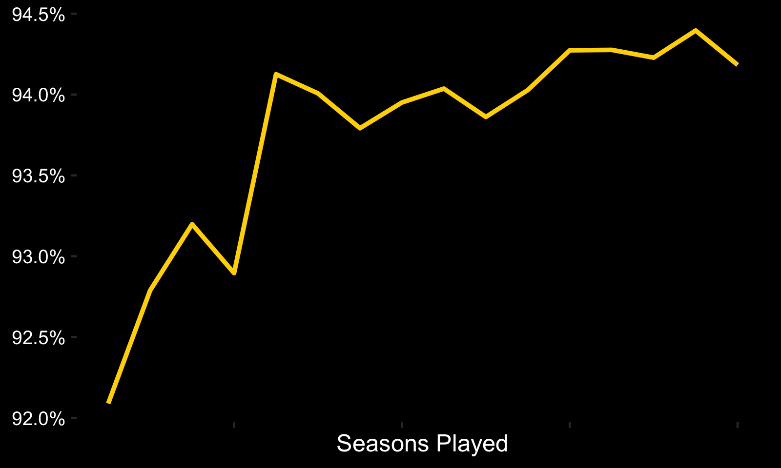
Weighting careers by attempts gives the most established goalies the greatest influence. Weighting careers equally lets very short, noisy careers shape the population distribution. Dropping those careers avoids the noise but discards nearly 30% of the players, despite losing less than 1% of attempts. None of those choices is neutral.
For a decision tool applied to active goalies, final career workload cannot be used as an ordinary predictor because it is not yet known. This is the point of departure.
Combining priors
One pragmatic solution is a mixture of two population priors: one estimated from careers below 1,500 attempts and one from careers at or above 1,500. The weight assigned to the long-career prior changes as the goalie accumulates attempts and performance information.
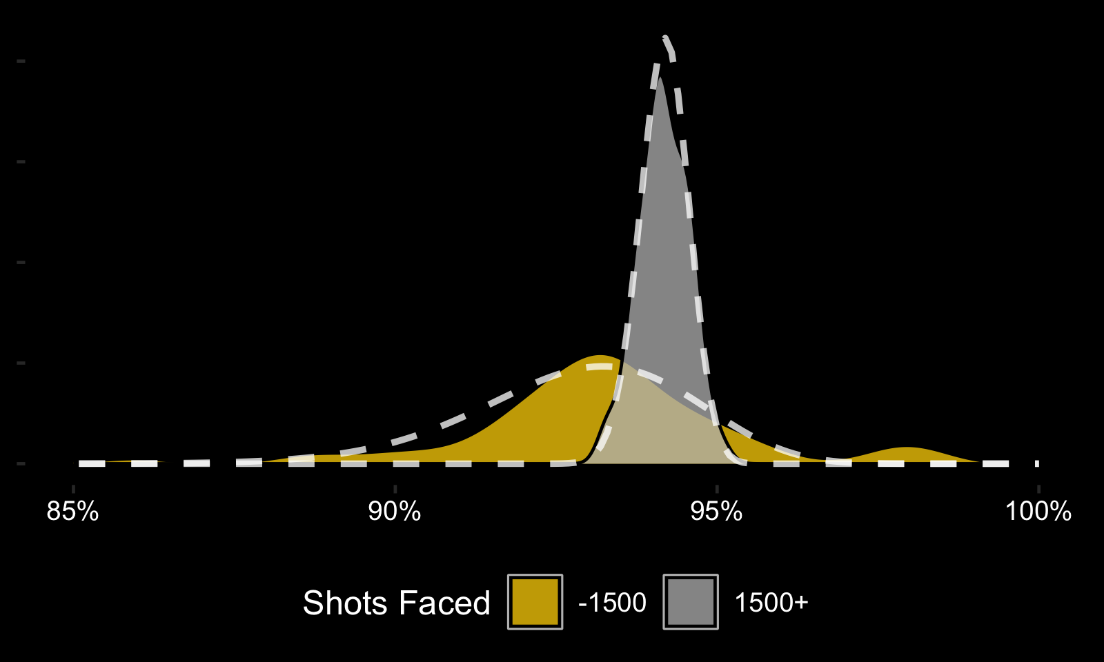
I estimate that weight with a logistic regression of eventual long-career status on current cumulative attempts and AdjSV%. The fitted probability answers a practical question: given what we know now, how likely is this goalie to finish with at least 1,500 attempts?
The model appears reasonably calibrated within this historical sample:
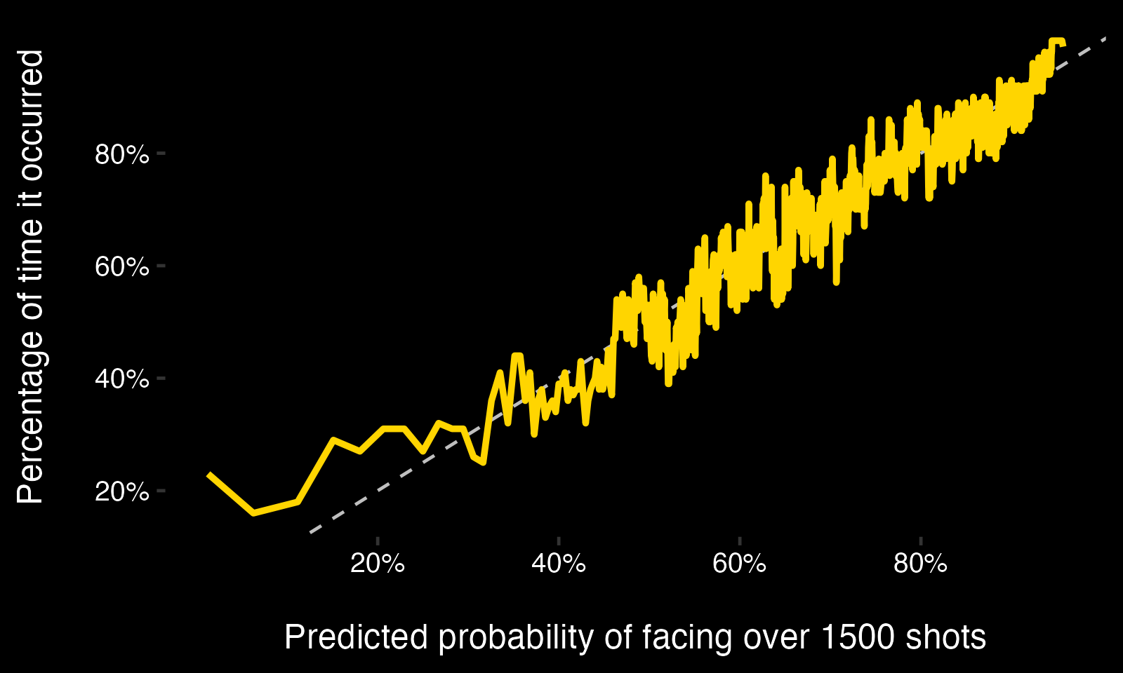
Let \(\pi_i\) be the predicted probability of a long career, \(A_i=N_i\mathrm{AdjSV}_i\) the fractional adjusted non-goal count, and \((\alpha_L,\beta_L)\) and \((\alpha_S,\beta_S)\) the long- and short-career beta parameters. The posterior estimate becomes:
\[ \boxed{ \widehat{\theta}_i = \pi_i \frac{\alpha_L+A_i}{\alpha_L+\beta_L+N_i} + (1-\pi_i) \frac{\alpha_S+A_i}{\alpha_S+\beta_S+N_i} } \]
This is a useful adaptive estimator, but not yet a fully generative model of ability and career survival. Because current performance helps determine \(\pi_i\) and also enters the posterior update, a future version should estimate opportunity and performance jointly.
CONTEXTUALIZING EXPERIENCE
Goalies in the analysis
Any fixed observation window cuts through some careers. In the 2007–2022 sample, some goalies enter near the end of the window while others began long before it. To compare complete career paths, I restrict this section to goalies whose observed careers both begin after 2007 and end before 2022. That leaves a narrower and selected population, but avoids mistaking the edge of the dataset for the beginning or end of a career.
The analysis population changes as follows:
- The goalie population drops from 314 to 155.
- Mean career attempts drop from 4,207 to 3,133.
- Shot-weighted AdjSV% remains .943; the unweighted goalie mean falls from .936 to .930.
Career length
The complete-career sample remains dominated by short NHL careers:
25% of goalies faced about 33 shots or less (!).
50% of goalies faced 202 shots or less (that’s about 7 games).
75% of goalies faced 3,531 shots or less.
40% of goalies played only one season.
74% of goalies played five seasons or less.
91% of goalies played twelve seasons or less.
The familiar long NHL career is therefore not the typical outcome. More importantly, experience and ability cannot be interpreted separately: performance affects whether a goalie receives the opportunity to become experienced.
The empirical Bayes estimate combines performance and sample size at each point in a career. I call the posterior mean pAdjSV% and recalculate it after every attempt. To compare paths, I group goalies by their eventual career workload:
- fewer than 300 attempts;
- 300–1,499 attempts;
- 1,500–5,999 attempts;
- 6,000 or more attempts.
\[ \mathrm{pAdjSV}_{i,n} = \mathbb{E}\!\left[\theta_i\mid D_{i,1:n}\right] \]
As an example, Braden Holtby’s pAdjSV% after facing various attempt totals in the reconstructed mixture model:
- 1 attempt: 0.9363
- 1,000 attempts: 0.9436
- 5,000 attempts: 0.9452
- 10,000 attempts: 0.9486
- 15,000 attempts: 0.9484
- 19,555 attempts: 0.9457
Among goalies who finish between 1,500 and 5,999 attempts, half end below the population benchmark. Their group trajectory also declines later in the observed career. These are commonly backup-sized workloads—roughly 600–1,000 attempts per season—but the pattern is descriptive. It combines aging, role, selection, and regression after a strong enough start to earn continued work.
To get a clearer sense of the dynamics described above, let’s take the group average pAdjSV% through each shot faced.
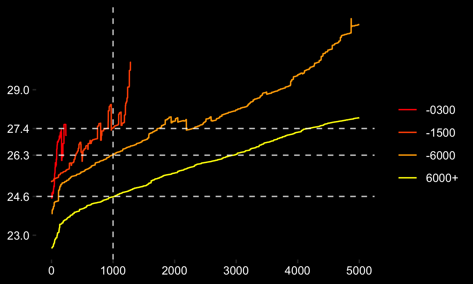
The grouped trajectories make the selection process clearer, but they do not identify its cause. The sub-300 group is too small and noisy to support much interpretation. The 300–1,499 group declines quickly, consistent with teams reducing opportunities after poor results. The 1,500–5,999 group begins above the others through roughly the first 1,000 attempts and then fades. That shape could reflect early randomness, aging, changing roles, or the conditioning on eventual career length itself.
Age provides one piece of that explanation. The final plot replaces pAdjSV% with average age for the same workload groups.
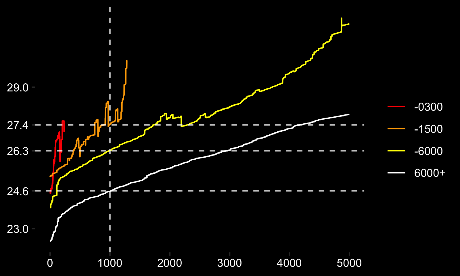
Goalies in the 1,500–5,999 group are roughly 1.5 years older than the 6,000-plus group at comparable career workloads. Much of that difference lies between ages 23 and 27, where the estimated age curve is still moving. Age can therefore explain part of the divergence, but not all of it; role and selection remain entangled with the trajectories.
Footnotes
Unlike conventional save percentage, it includes attempts which miss the net as non-goal outcomes. This may capture some goalie influence on whether an attempt reaches the net.↩︎