Goalie Consistency
Note / Hockey
5 min read
Goaltenders make up the least predictable position in hockey. Their behaviour confounds analysts and casual fans alike. It isn’t uncommon for a good goalie to have a below-replacement season, or for an unknown goalie to arrive and dominate the league for a stretch of time. They’re voodoo, it’s often said.
Consistency can mean two different things here. A goalie can vary from game to game, following a strong start with a weak one. They can also vary within a game, bunching their goals against into streaks rather than spreading them evenly through the season. The two ideas sound similar, but they do not produce the same result.
Which goalie would you choose?
Imagine a league where every skater and goalie is equally skilled. Five goalies have the same average ability, but different levels of game-to-game variation. Goalie A is expected to allow three goals every night. Goalie B is a little better than average in half of their games and a little worse in the other half. The spread grows through goalies C, D and E, while the season-long average remains fixed.
Goals are drawn from a Poisson distribution around each game’s expectation. Ten thousand 82-game seasons produce the following results:
EXPECTED STANDING POINTS
| Goalie | Game-to-game variation | Mean | SD |
|---|---|---|---|
| A | None | 89.05 | 8.38 |
| B | Slight | 89.63 | 8.31 |
| C | Moderate | 91.01 | 7.95 |
| D | High | 92.68 | 7.29 |
| E | Highest | 94.70 | 6.26 |
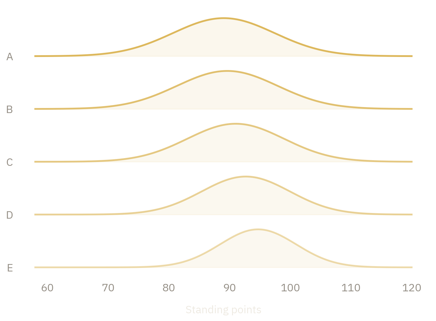
The less consistent goalies earn more standing points on average. This feels backwards until the conversion from goals to wins is considered. A goalie expected to allow one goal in one game and five in another gives their team one very strong chance to win. A goalie expected to allow three in both games gives the team two middling chances. The bad night can only lose one game; the good night can turn the other into a near-certain win.
The difference between A and E is about five points, or 2.4 wins, over a full season. Their season totals are also less variable because the result of each high- or low-expectation game becomes more certain.
This is a property of the standings system, not a strategy a goalie can follow. A goalie cannot choose to be inconsistent. It only says that equal average performance need not produce equal expected points when that performance is distributed differently between games.
What about shot-to-shot consistency?
A season can also be written as a sequence of saves and goals:
0 0 0 0 1 0 0 0 1 0
Let \(s_{ig}\) be the number of saves made by goalie \(i\) between goals \(g-1\) and \(g\), and let \(S_i\) be their total saves. The share of the season contained in each run is
\[ x_{ig}=\frac{s_{ig}}{S_i}. \]
A simple streakiness score is the negative of conventional Shannon entropy:
\[ C_i=\frac{1}{G_i+1}\sum_{g=1}^{G_i+1}x_{ig}\log(x_{ig}), \]
where \(G_i\) is the number of goals allowed. Larger values mean the saves are concentrated in fewer, longer runs. Because the raw score depends on both workload and save percentage, each season is compared with 10,000 shuffled versions of itself. Its percentile says how unusually streaky the observed ordering was, without changing the shots or the number of goals.
The same exercise can be used as a simulation. Shuffle the outcomes from a .900 save-percentage season into 10,000 different sequences, split each sequence into games, and calculate both its streakiness percentile and standing points.
SHOT ORDER AND STANDING POINTS
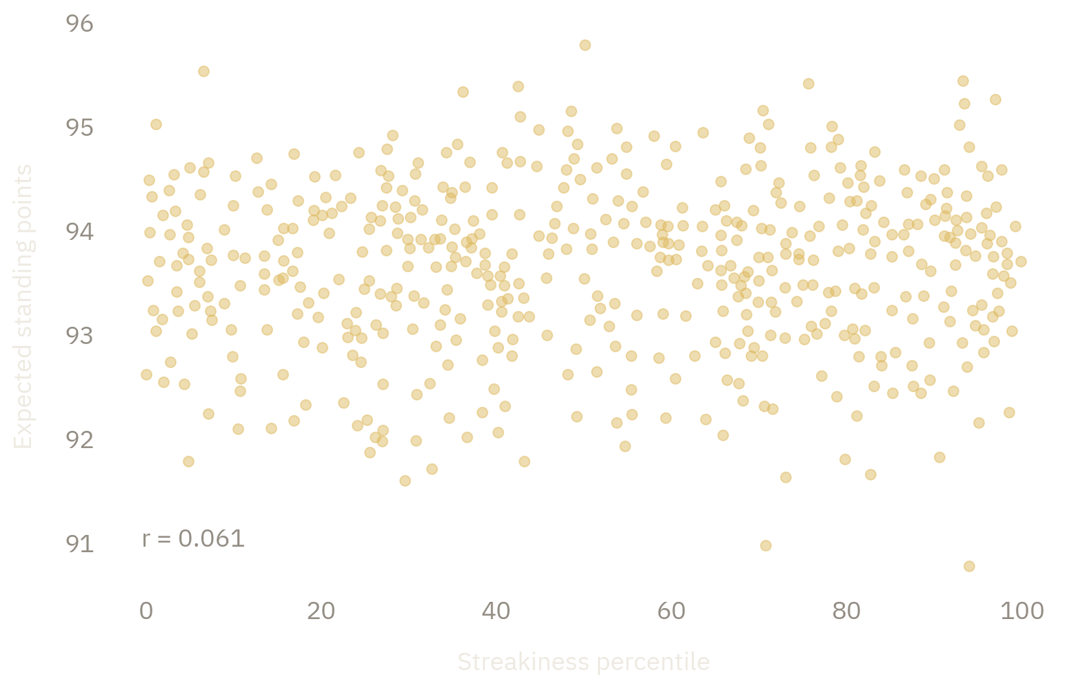
There is no relationship. Unlike game-to-game changes in expected ability, rearranging the order of saves and goals within an otherwise identical season does not meaningfully change expected points.
Shots are not equal
The binary version treats a point shot through traffic and an uncontested shot from the boards as equivalent. Expected goals provide the natural weight. If a goalie allows \(G_i\) goals on shots with expected-goal probabilities \(p_j\), first scale each probability so the simulated season retains the goalie’s observed performance:
\[ p_j^*=p_j\frac{G_i}{\sum_j p_j}. \]
Thatcher Demko, for example, allowed 99 goals against 105.7 expected in 2020. A shot originally worth 14% becomes \(0.14(99/105.7)=13.1\%\). The sequence can then be simulated with these adjusted probabilities.
For the NHL data, replace the number of saves in a run with the expected-goal value of those saves. If \(\mathcal{R}_{ig}\) is the set of saved shots between two goals, then
\[ x_{ig}^{xG}=\frac{\sum_{j\in\mathcal{R}_{ig}}p_j^*}{\sum_j p_j^*}, \]
and use \(x_{ig}^{xG}\) in the same streakiness score. Again, the result is expressed as a percentile against shuffled seasons with the same shots and overall performance.
The sample includes seasons of at least 800 shots. Career comparisons require at least five such seasons.
STREAKINESS AND PERFORMANCE
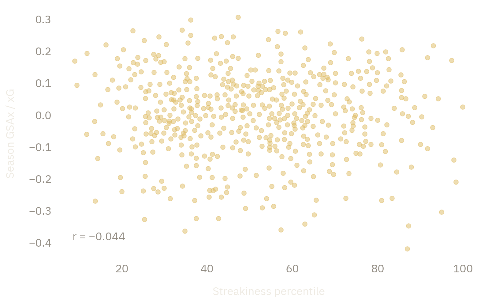
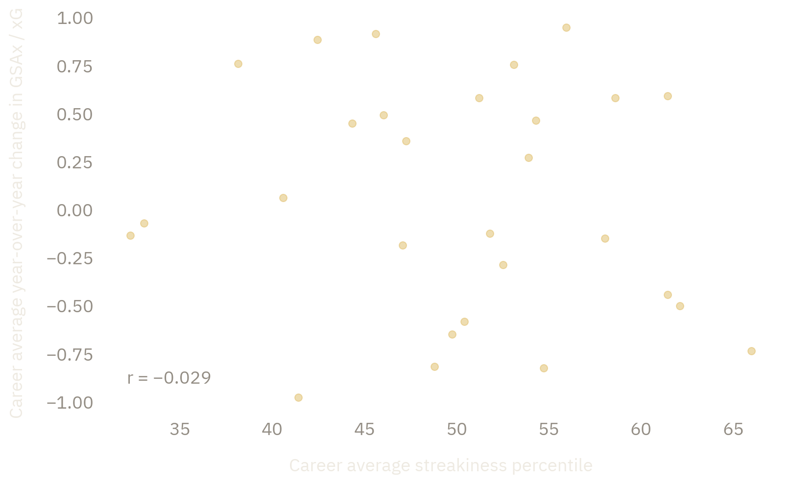
Better seasons are not more or less streaky. More importantly, streakiness does not persist across a goalie’s career:
STREAKINESS AND YEAR-TO-YEAR CHANGE
Does consistency matter?
Game-to-game variation can change expected standing points even when average goalie ability is held fixed. Shot-to-shot streakiness does not appear to do the same, nor does it identify better goalies or more stable careers.
This is the useful distinction. A run of goals against is visible and frustrating, but that does not make it a repeatable property of the goalie. In this sample, “inconsistent” describes the order in which the outcomes arrived more readily than it describes a stable skill.